1. Naive Bayes 算法

1.1 算法原理

$NaiveBayes$ 算法基于贝叶斯定理和特征条件独立假设的分类方法，通过从训练集数据中习得联合概率分布 $P(X,Y)$，进一步得出贝叶斯分类器，依据该分类器对未知类别的数据进行分类。

1.2 算法流程

Step 1. 从训练集中学习先验概率 P ( Y = c k ) , k = 1 , 2 , ⋯ , K P(Y=c_k),k=1,2,\cdots,K P(Y=ck​),k=1,2,⋯,K
Step 2. 从训练集中学习条件概率 P ( X = x ∣ Y = c k ) , k = 1 , 2 , ⋯ , K P(X=x|Y=c_k),k=1,2,\cdots,K P(X=x∣Y=ck​),k=1,2,⋯,K
Step 3. 得到贝叶斯分类器 y = arg ⁡ max ⁡ c k P ( Y = c k ) ∏ j P ( X ( j ) = x ( j ) ∣ Y = c k ) y=\arg\underset{c_k}{\max}P(Y=c_k)\underset{j}{\prod}P(X^{(j)}=x^{(j)}|Y=c_k) y=argck​max​P(Y=ck​)j∏​P(X(j)=x(j)∣Y=ck​)
Step 4. 用贝叶斯分类器对未知类别数据进行分类

1.3 公式推导

1.3.1 先验概率和条件概率

先验概率和条件概率可以用参数估计的方式从训练集中习得

• 极大似然估计
  使用极大似然估计时，这两个概率如下：
  P ( Y = c k ) = ∑ i = 1 N I ( y i = c k ) N , k = 1 , 2 , ⋯ , K P ( X ( j ) = a j l ∣ Y = c k ) = ∑ i = 1 N I ( x i ( j ) = a j l , y i = c k ) ∑ i = 1 N I ( y i = c k ) , j = 1 , 2 , ⋯ , n ; l = 1 , 2 , ⋯ , S j ; k = 1 , 2 , ⋯ , K \begin{aligned}P(Y=c_k) & =\frac{\sum\limits_{i=1}^NI(y_i=c_k)}{N},k=1,2,\cdots,K\\ P(X^{(j)}=a_{jl}|Y=c_k) & =\frac{\sum\limits_{i=1}^NI(x_i^{(j)}=a_{jl},y_i=c_k)}{\sum_{i=1}^NI(y_i=c_k)},j=1,2,\cdots,n;l=1,2,\cdots,S_j;k=1,2,\cdots,K\end{aligned} P(Y=ck​)P(X(j)=ajl​∣Y=ck​)​=Ni=1∑N​I(yi​=ck​)​,k=1,2,⋯,K=∑i=1N​I(yi​=ck​)i=1∑N​I(xi(j)​=ajl​,yi​=ck​)​,j=1,2,⋯,n;l=1,2,⋯,Sj​;k=1,2,⋯,K​
• 贝叶斯估计
  使用极大似然估计时，可能会出现所要估计的概率值为 $0$ 的情况，会影响到后验概率的计算结果，因此，使用贝叶斯估计来解决这个问题。
  使用贝叶斯估计时，这两个概率如下：
  P λ ( Y = c k ) = ∑ i = 1 N I ( y i = c k ) + λ N + K λ , k = 1 , 2 , ⋯ , K P λ ( X ( j ) = a j l ∣ Y = c k ) = ∑ i = 1 N I ( x i ( j ) = a j l , y i = c k ) + λ ∑ i = 1 N I ( y i = c k ) + S j λ , j = 1 , 2 , ⋯ , n ; l = 1 , 2 , ⋯ , S j ; k = 1 , 2 , ⋯ , K \begin{aligned}P_{\lambda}(Y=c_k) & =\frac{\sum\limits_{i=1}^NI(y_i=c_k)+\lambda}{N+K\lambda},k=1,2,\cdots,K\\ P_{\lambda}(X^{(j)}=a_{jl}|Y=c_k) & =\frac{\sum\limits_{i=1}^NI(x_i^{(j)}=a_{jl},y_i=c_k)+\lambda}{\sum_{i=1}^NI(y_i=c_k)+S_j\lambda},j=1,2,\cdots,n;l=1,2,\cdots,S_j;k=1,2,\cdots,K\end{aligned} Pλ​(Y=ck​)Pλ​(X(j)=ajl​∣Y=ck​)​=N+Kλi=1∑N​I(yi​=ck​)+λ​,k=1,2,⋯,K=∑i=1N​I(yi​=ck​)+Sj​λi=1∑N​I(xi(j)​=ajl​,yi​=ck​)+λ​,j=1,2,⋯,n;l=1,2,⋯,Sj​;k=1,2,⋯,K​
• 注：
  • 当贝叶斯估计中，$\lambda =0$ 时，就是极大似然估计
  • 当 $\lambda =1$ 时，则称为拉普拉斯平滑

1.3.2 贝叶斯分类器

1.求联合概率分布
公式 $P(X,Y)=P(X|Y)P(Y)$ 使得我们能够根据先验概率 $P(Y)$ 和条件概率 $P(X|Y)$ 习得联合概率分布
2.求后验概率
P ( Y ∣ X ) = P ( X , Y ) P ( X ) = P ( X ∣ Y ) P ( Y ) P ( X ) P(Y|X)=\frac{P(X,Y)}{P(X)}=\frac{P(X|Y)P(Y)}{P(X)} P(Y∣X)=P(X)P(X,Y)​=P(X)P(X∣Y)P(Y)​
3.贝叶斯分类器
因为 $NB$ 算法对条件概率做了条件独立性的假设，即数据的属性之间假设为独立的，因而有
P ( X = x ∣ Y = c k ) = P ( X ( 1 ) = x ( 1 ) , ⋯ , X ( n ) = x ( n ) ∣ Y = c k ) = ∏ j = 1 n P ( X ( j ) = x ( j ) ∣ Y = c k ) P(X=x|Y=c_k)=P(X^{(1)}=x^{(1)},\cdots,X^{(n)}=x^{(n)}|Y=c_k)=\prod_{j=1}^nP(X^{(j)}=x^{(j)}|Y=c_k) P(X=x∣Y=ck​)=P(X(1)=x(1),⋯,X(n)=x(n)∣Y=ck​)=j=1∏n​P(X(j)=x(j)∣Y=ck​)
再结合全概率公式 P ( X ) = ∑ i = 0 K P ( X ∣ Y i ) P ( Y i ) P(X)=\sum\limits_{i=0}^KP(X|Y_i)P(Y_i) P(X)=i=0∑K​P(X∣Yi​)P(Yi​)可以推出
P ( Y = c k ∣ X = x ) = P ( Y = c k ) ∏ j P ( X ( j ) = x ( j ) ∣ Y = c k ) ∑ k P ( Y = c k ) ∏ j P ( X ( j ) = x ( j ) ∣ Y = c k ) , k = 1 , 2 , ⋯ , K P(Y=c_k|X=x)=\frac{P(Y=c_k)\underset{j}{\prod}P(X^{(j)}=x^{(j)}|Y=c_k)}{\underset{k}{\sum}P(Y=c_k)\underset{j}{\prod}P(X^{(j)}=x^{(j)}|Y=c_k)},k=1,2,\cdots,K P(Y=ck​∣X=x)=k∑​P(Y=ck​)j∏​P(X(j)=x(j)∣Y=ck​)P(Y=ck​)j∏​P(X(j)=x(j)∣Y=ck​)​,k=1,2,⋯,K
对于同一条数据的每个分类，其实上式的分母值都是相同的的，因此我们可以直接忽略分母，凭分子就可以判断该数据属于哪一类的概率更大了，因此得到贝叶斯分类器
y = arg ⁡ max ⁡ c k P ( Y = c k ) ∏ j P ( X ( j ) = x ( j ) ∣ Y = c k ) y=\arg\max_{c_k}P(Y=c_k)\prod_jP(X^{(j)}=x^{(j)}|Y=c_k) y=argck​max​P(Y=ck​)j∏​P(X(j)=x(j)∣Y=ck​)
在计算机处理的时候，需要对上式取对数，以避免溢出，即
y = arg ⁡ max ⁡ c k log ⁡ P ( Y = c k ) ∑ j log ⁡ P ( X ( j ) = x ( j ) ∣ Y = c k ) y=\arg\max_{c_k}\log P(Y=c_k)\sum_j\log P(X^{(j)}=x^{(j)}|Y=c_k) y=argck​max​logP(Y=ck​)j∑​logP(X(j)=x(j)∣Y=ck​)
4.拉普拉斯平滑
若采用极大似然估计，则会存在一个一票否决的问题，即只要连乘式子中有一个连乘因子为 $0$，那么要估计的概率值就是 $0$。解决方法就是用贝叶斯估计，通过对概率分布加上一个大于 $0$ 的参数 $\lambda$ 来避免连乘因子为 $0$ 的可能性，我们取 $\lambda =1$，即拉普拉斯平滑。

2. 程序

2.1 读入数据

第一步是读取数据，有两个方法，第一个是从给出文件名的 arff 文件中读取数据，第二个是从一个 Instances 数据结构中读取文件。两者都将数据存储在一个名为 dataset 的 Instances 数据结构中，并设定类别属性，记录条件属性，实例，类别的数目。区别就是第一个方法在读入数据失败时会抛出异常。

	/****************************** The constructor.** @param paraFilename The given file.****************************/public NaiveBayes(String paraFilename) {dataset = null;try {FileReader fileReader = new FileReader(paraFilename);dataset = new Instances(fileReader);fileReader.close();} catch (Exception ee) {System.out.println("Cannot read the file: " + paraFilename + "\r\n" + ee);System.exit(0);} // Of trydataset.setClassIndex(dataset.numAttributes() - 1);numConditions = dataset.numAttributes() - 1;numInstances = dataset.numInstances();numClasses = dataset.attribute(dataset.numAttributes() - 1).numValues();} // Of the constructor/****************************** The constructor.** @param paraFilename The given file.****************************/public NaiveBayes(Instances paraInstances) {dataset = paraInstances;dataset.setClassIndex(dataset.numAttributes() - 1);numConditions = dataset.numAttributes() - 1;numInstances = dataset.numInstances();numClasses = dataset.attribute(dataset.numAttributes() - 1).numValues();} // Of the constructor

2.2 设定数据类型

根据给定的类型来确定数据类型，不过今天只处理符号型数据。

	/****************************** Set the data type.****************************/public void setDataType(int paraDataType) {dataType = paraDataType;} // Of setDataType

2.3 从训练集学习先验概率和条件概率

2.3.1 先验概率

遍历所有数据，统计他们的类别，遇到一个 tempClassValue 的数据，就将 tempCounts[tempClassValue] 的值增一。统计了各类别的实例数目后，根据前文推导的公式依次计算每一类的先验概率即可。

	/****************************** Calculate the class distribution with Laplacian smooth.****************************/public void calculateClassDistribution() {classDistribution = new double[numClasses];classDistributionLaplacian = new double[numClasses];double[] tempCounts = new double[numClasses];for(int i = 0; i < numInstances; ++i) {int tempClassValue = (int) dataset.instance(i).classValue();tempCounts[tempClassValue]++;} // Of for ifor(int i = 0; i < numClasses; ++i) {classDistribution[i] = tempCounts[i] / numInstances;classDistributionLaplacian[i] = (tempCounts[i] + 1) / (numInstances + numClasses);} // Of for iSystem.out.println("Class distribution: " + Arrays.toString(classDistribution));System.out.println("Class distribution Laplacian: " + Arrays.toString(classDistributionLaplacian));} // Of calculateClassDistribution

2.3.2 条件概率

先说一下这里的数据结构，也就是三维数组 conditionalCounts 和 conditionalProbabilitiesLaplacian，以前者为例 conditionalCounts[i][j][tempValue] ，代表第 $i$ 条数据的第 $j$ 个属性的第 tempValue 种取值出现的次数。由于每个属性的可能取值个数不同，因此这实际上是一个参差不齐的“三维数组”，后者在前者的基础上保存拉普拉斯平滑下计算出的条件概率。
这个方法分三步，第一步分配空间，第二步遍历每条数据的每个属性，统计它们出现的次数，此外还要统计属于各类的实例个数，第三步就是根据推导的公式计算条件概率。

	/****************************** Calculate the conditional probabilities with Laplacian smooth.****************************/public void calculateConditionalProbabilities() {conditionalCounts = new double[numClasses][numConditions][];conditionalProbabilitiesLaplacian = new double[numClasses][numConditions][];// Allocate spacefor(int i = 0; i < numClasses; ++i) {for(int j = 0; j < numConditions; ++j) {int tempNumValues = (int) dataset.attribute(j).numValues();conditionalCounts[i][j] = new double[tempNumValues];conditionalProbabilitiesLaplacian[i][j] = new double[tempNumValues];} // Of for j} // Of for i// Count the numbersint[] tempClassCounts = new int[numClasses];for(int i = 0; i < numInstances; ++i) {int tempClass = (int) dataset.instance(i).classValue();tempClassCounts[tempClass]++;for(int j = 0; j < numConditions; ++j) {int tempValue = (int) dataset.instance(i).value(j);conditionalCounts[tempClass][j][tempValue]++;} // Of for j} // Of for i// Now for the real probability with Laplacianfor(int i = 0; i < numClasses; ++i) {for(int j = 0; j < numConditions; ++j) {int tempNumValues = (int) dataset.attribute(j).numValues();for(int k = 0; k < tempNumValues; ++k) {conditionalProbabilitiesLaplacian[i][j][k] = (conditionalCounts[i][j][k] + 1) / (tempClassCounts[i] + tempNumValues);} // Of for k} // Of for j} // Of for iSystem.out.println("Conditional probabilities: " + Arrays.deepToString(conditionalCounts));} // Of calculateConditionalProbabilities

2.4 分类

计算出先验概率和条件概率后，贝叶斯分类器也就已经得出，因此接下来就应用此分类器进行分类。
这里有三个方法，第一个 classify 不接受任何参数，而是对每条数据调用重载后的 classify，这有助于对外提供清晰的接口。第二个方法根据数据类型来决定调用哪个分类方法，但由于今天只处理符号型，所以删除了 else if 的部分。第三个方法就是对符号型数据分类的方法，根据推出的贝叶斯分类器的公式，计算实例 $x$ 属于每一类的概率，然后以概率最大的类为输出。

	/****************************** Classify all instances, the results are stored in predicts[].****************************/public void classify() {predicts = new int[numInstances];for(int i = 0; i < numInstances; ++i) {predicts[i] = classify(dataset.instance(i));} // Of for if} // Of classify/****************************** Classify an instances.****************************/public int classify(Instance paraInstance) {if(dataType == NOMINAL) {return classifyNominal(paraInstance);} // Of ifreturn -1;} // Of classify/****************************** Classify an instances with nominal data.****************************/public int classifyNominal(Instance paraInstance) {// Find the biggest onedouble tempBiggest = -10000;int resultBestIndex = 0;for(int i = 0; i < numClasses; ++i) {double tempPseudoProbability = Math.log(classDistributionLaplacian[i]);for(int j = 0; j < numConditions; ++j) {int tempAttributeValue = (int) paraInstance.value(j);tempPseudoProbability += Math.log(conditionalProbabilitiesLaplacian[i][j][tempAttributeValue]);} // Of for jif(tempBiggest < tempPseudoProbability) {tempBiggest = tempPseudoProbability;resultBestIndex = i;} // Of if} // Of for ireturn resultBestIndex;} // Of classifyNominal

2.5 计算精确度

挨个对比实例真实的类别和我们用贝叶斯分类器所得到的类别，统计分类正确的实例数，计算其占总实例数的比值作为输出。

	/****************************** Compute accuracy.****************************/public double computeAccuracy() {double tempCorrect = 0;for(int i = 0; i < numInstances; ++i) {if(predicts[i] == (int) dataset.instance(i).classValue()) {tempCorrect++;} // Of if} // Of for idouble resultAccuracy = tempCorrect / numInstances;return resultAccuracy;} // Of computeAccuracy

2.6 数据测试

用 mushroom 数据集来进行测试。

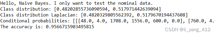
	/****************************** Test nominal data.****************************/public static void testNominal() {System.out.println("Hello, Naive Bayes. I only want to test the nominal data.");String tempFilename = "G:/Program Files/Weka-3-8-6/data/mushroom.arff";NaiveBayes tempLearner = new NaiveBayes(tempFilename);tempLearner.setDataType(NOMINAL);tempLearner.calculateClassDistribution();tempLearner.calculateConditionalProbabilities();tempLearner.classify();System.out.println("The accuracy is: " + tempLearner.computeAccuracy());} // Of testNominal/****************************** Test this class.** @param args Not used now.****************************/public static void main(String[] args) {testNominal();} // Of main

测试结果如下，准确度在 0.95 的样子。

本文来自互联网用户投稿，文章观点仅代表作者本人，不代表本站立场，不承担相关法律责任。如若转载，请注明出处。 如若内容造成侵权/违法违规/事实不符，请点击【内容举报】进行投诉反馈！