ggplot2的主题设置与一页多图
图形的视觉呈现由数据和非数据部分决定,主题系统控制着图形中的非数据元素外观,包括标题、坐标轴标签、图例标签等文字调整,以及网格线、背景、轴须的颜色搭配等。
ggplot2的绘图策略是首先确定数据如何展示,然后利用主题系统对细节进行渲染。
一、内置主题
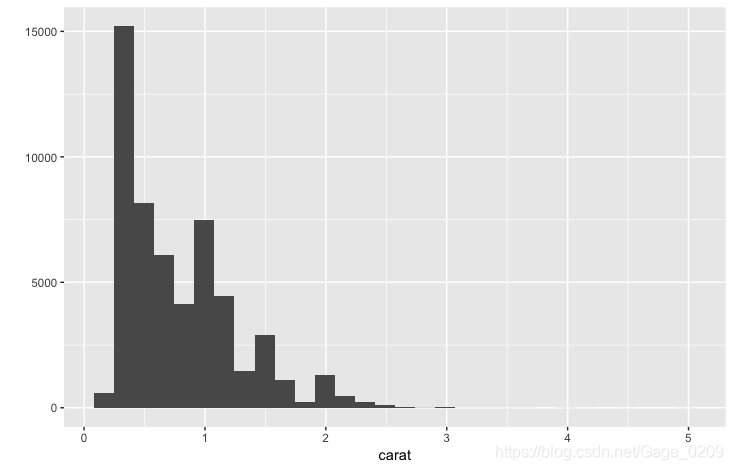
内置主题有两种:默认的theme_gray()和theme_bw()
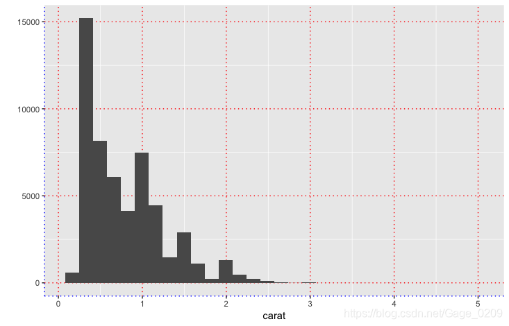
#默认为theme_gray():淡灰色背景+白色网格线
hgram <- qplot(carat, data = diamonds)
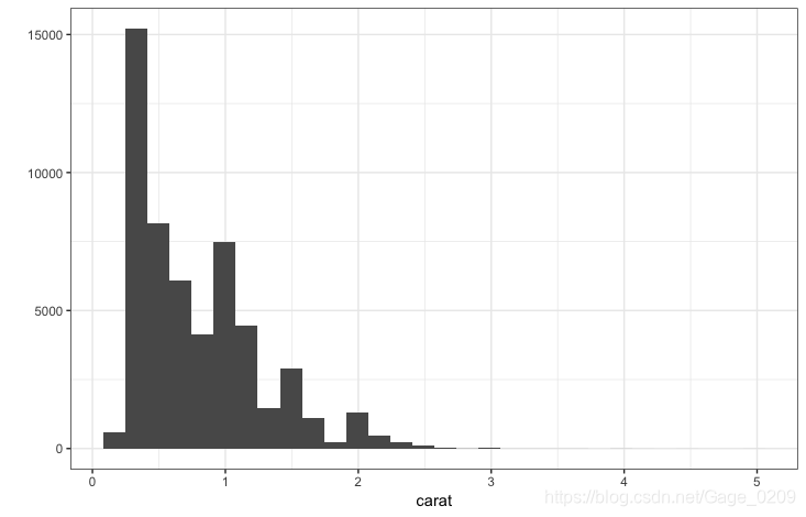
#另一个固定主题theme_bw():白色背景+灰色网格线
#局部设置,只对这个图有效
hgram + theme_bw()#全局性设置
##theme_set()返回先前的主题,可储存以备后用
previous_theme <- theme_set(theme_bw()) #现在的主题被设置成theme_bw(),现在的主题被保存在previous_theme
hgram
#返回先前的主题
hgram + previous_theme
#永久性储存初始主题
theme_set(previous_theme)
二、主题元素和元素函数
(一) 主题元素
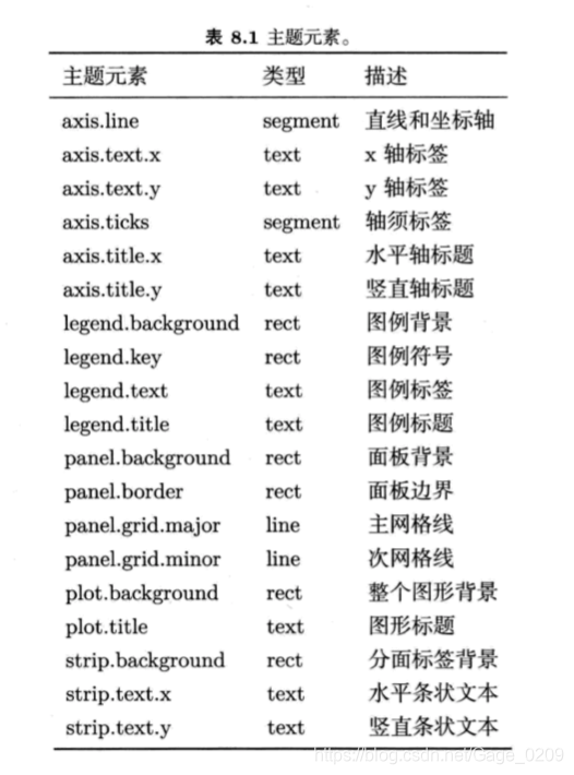
(二) 元素函数
内置的元素函数有四个基础类型:文本(text)、线条(lines)、矩形(rect)、空白(blank)
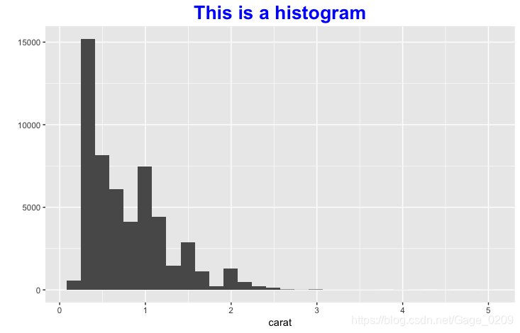
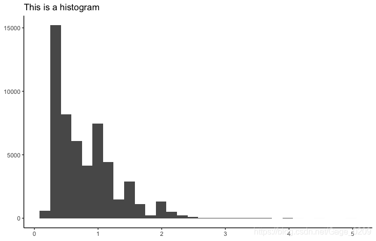
- element_text():绘制标签和标题
##element_text():绘制标签和标题
hgramt <- hgram + labs(title = 'This is a histogram')
hgramt + theme(plot.title = element_text(hjust = 0.5,#水平居中size = 20,#字体大小face = 'bold',#字体加粗colour = 'blue',#颜色angle = 0)) #标题旋转角度
2. element_line():绘制线条或线段
hgram + theme(panel.grid.major = element_line(colour = 'red',#主网格线颜色size = 0.5, #主网格线粗细linetype = 'dotted'), #主网格线线条类型axis.line = element_line(colour = 'blue', #坐标轴线条颜色size = 0.5, #坐标轴粗细linetype = 'dotted')) #坐标轴线条类型
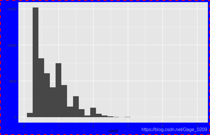
3. element_rect()绘制主要供背景使用的矩形
hgram + theme(plot.background = element_rect(fill = 'blue', #整个图形的背景填充颜色colour = 'red', #图形背景的边框颜色linetype = 'dotted', #图形背景的边框线条类型size = 2)) #图形背景边框的线条粗细
4. element_blank()空主题:可以删除我们不感兴趣的绘图元素
hgramt
last_plot() + theme(panel.grid.minor = element_blank(),  #删除次网格线panel.grid.major = element_blank(),  #删除主网格线panel.background = element_blank(),  #删除面板背景axis.title.x = element_blank(),      #删除水平轴标题axis.title.y = element_blank())		 #删除垂直轴标题
last_plot() + theme(axis.line = element_line())
三、存储输出
#ggsave函数
ggsave(filename, plot = last_plot(), device = NULL, path = NULL,scale = 1, width = NA, height = NA, units = c("in", "cm", "mm"),dpi = 300, limitsize = TRUE, ...)#path:设定图形存储的路径
#三个控制输出尺寸的参数:scale、width、height
##width和height设置绝对尺寸大小
##scale设置图形相对屏幕展示的尺寸大小
#对于光栅图,dpi控制图形的分辨率,默认300
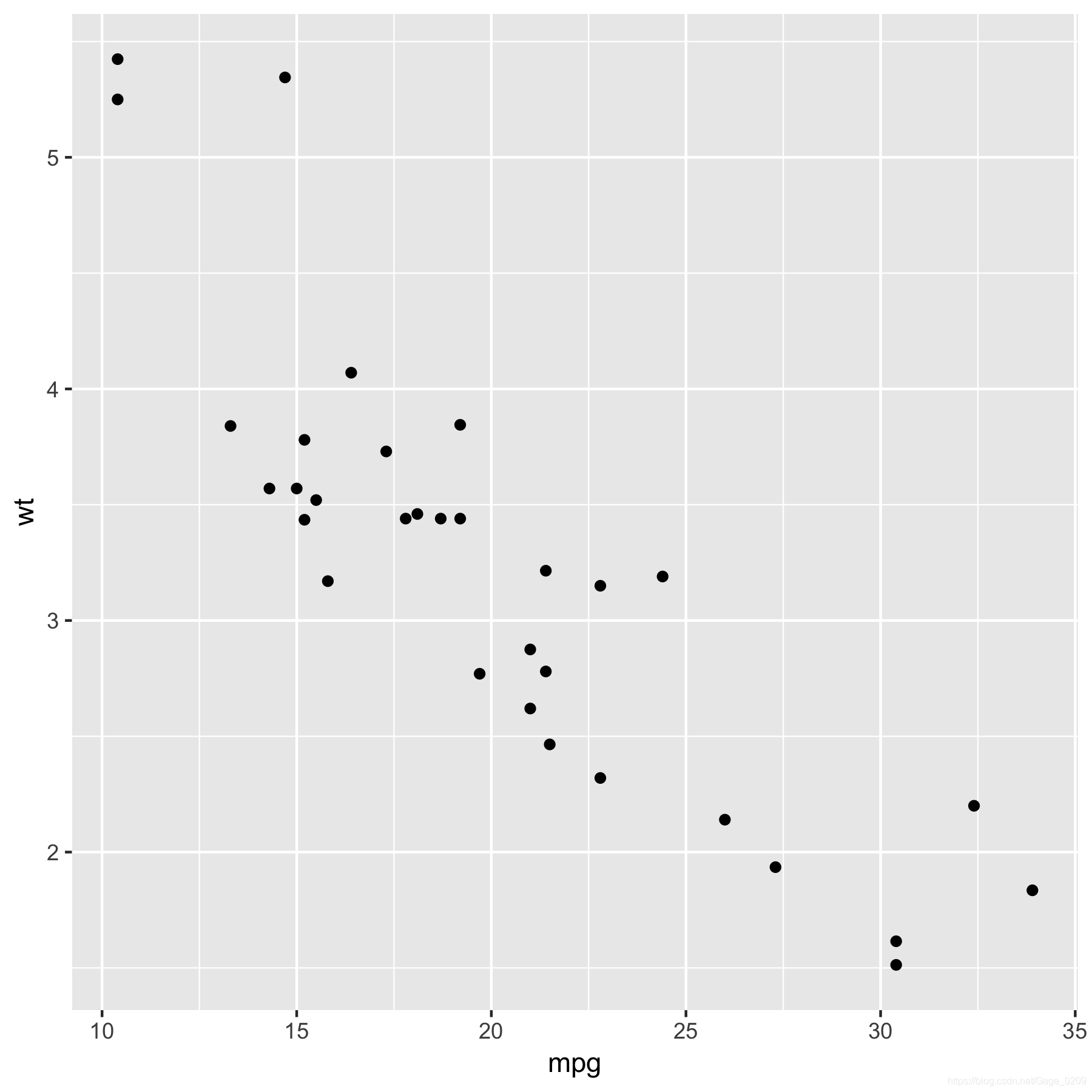
#可以修改为600,用于高分辨率输出qplot(mpg,wt, data = mtcars)
ggsave(file = 'output3.png', width = 6, height = 6,scale = 1)
将多幅图形存储到一个文件中
pdf(file = 'output5.pdf', width = 6, height = 6)
qplot(mpg, wt, data = mtcars)
qplot(wt, mpg, data = mtcars)
dev.off()
四、一页多图
(一) 子图
viewport(x = unit(0.5, "npc"), y = unit(0.5, "npc"),width = unit(1, "npc"), height = unit(1, "npc"),default.units = "npc", just = "centre",gp = gpar(), clip = "inherit",xscale = c(0, 1), yscale = c(0, 1),angle = 0,layout = NULL,layout.pos.row = NULL, layout.pos.col = NULL,name = NULL)
#将图形命名为变量
a <- qplot(date, unemploy, data = economics, geom = 'line')
b <- qplot(uempmed, unemploy, data = economics) + geom_smooth(se = F)
c <- qplot(uempmed, unemploy, data = economics, geom = 'path')
library(grid)
#x、y控制视图窗口的中心位置,默认定位在图形设备中心,即x=y=0.5
##占据整个图形设备的视图窗口
vp1 <- viewport(width = 1, height = 1, x = 0.5, y = 0.5)
vp1 <- viewport()
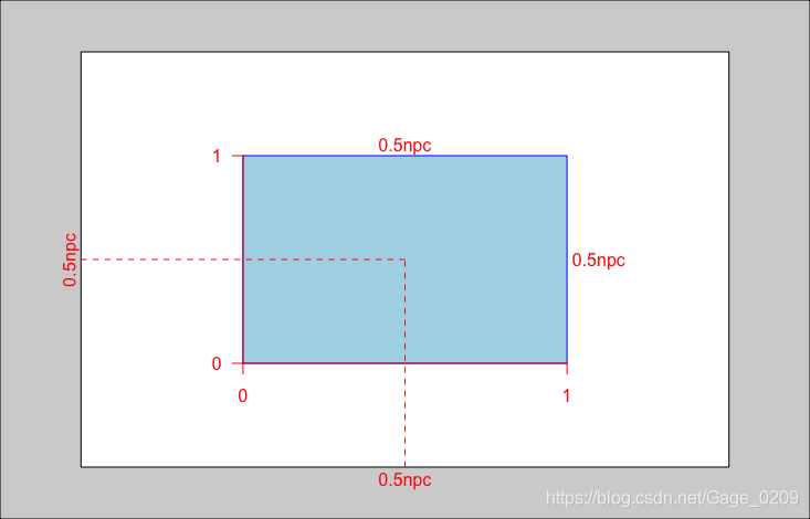
#也在中心位置,但视图窗口只占图形设备的一半宽度和高度
vp2 <- viewport(width = 0.5, height = 0.5, x = 0.5, y = 0.5)
vp2 <- viewport(width = 0.5, height = 0.5)
#查看创建的视图窗口
grid.show.viewport(vp2)
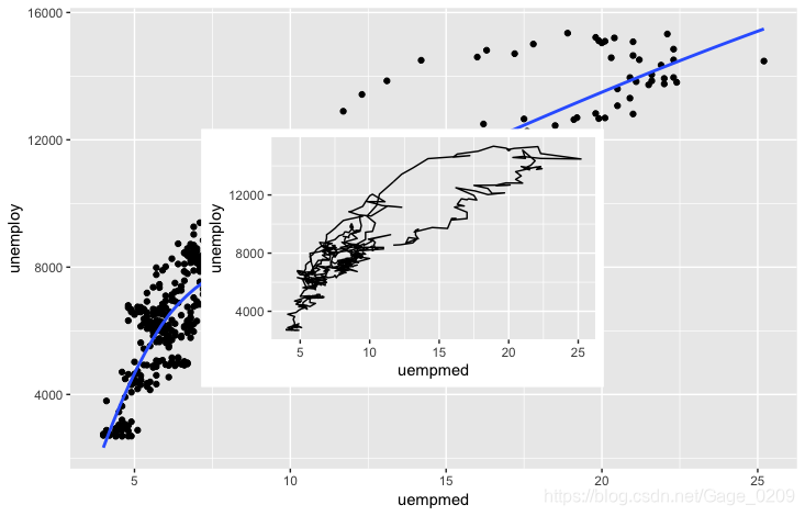
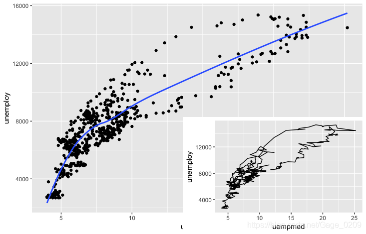
#以b图为基础,在中心插入子图c
b
print(c, vp = vp2)
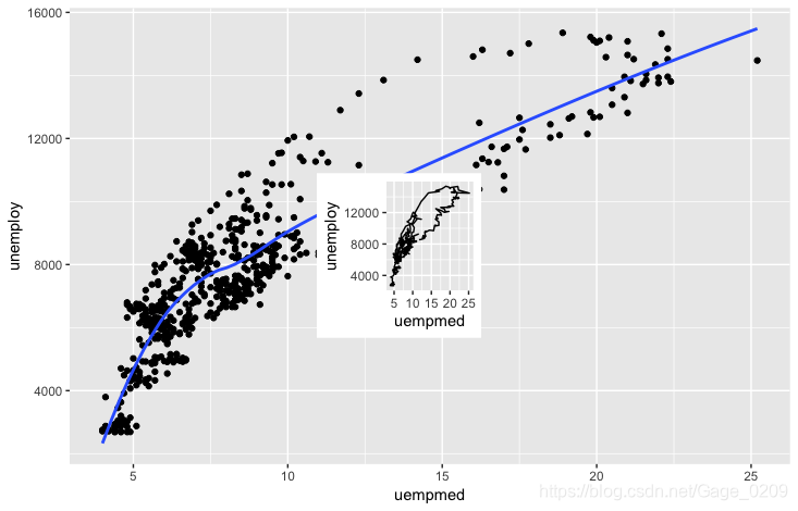
#在图形设备中心画一个4cm x 4cm的视图窗口
vp3 <- viewport(width = unit(4, "cm"), height = unit(4, "cm"))
b
print(c, vp = vp3)
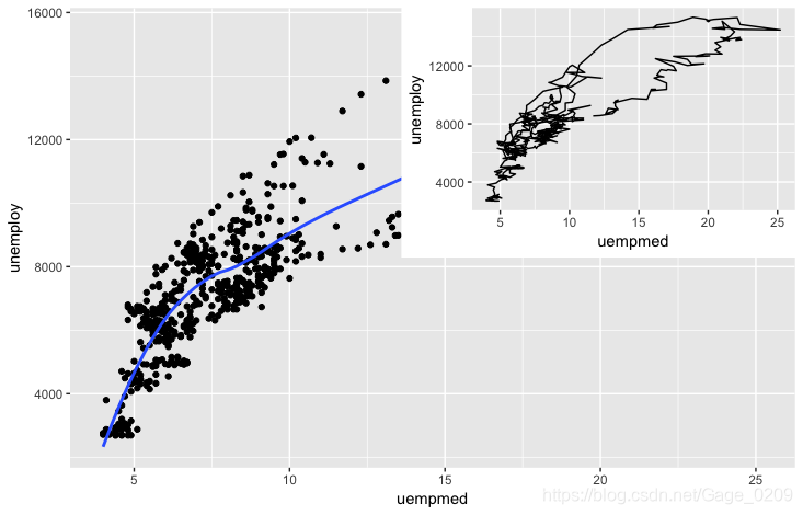
x、y控制视图窗口的中心位置,默认定位在图形设备中心,即x=y=0.5,若想调整图形的位置,需要通过just参数控制将图形放置在哪个边角,这里有一点要特别注意,just向量的第一个参数控制水平方向,第二个参数控制垂直方向
#在右上角的视图窗口,大小只有图形设备1/4
#注意:just向量的第一个参数控制水平方向,第二个参数控制垂直方向
vp4 <- viewport(x = 1, y = 1,width = 0.5, height = 0.5, just = c("right", "top"))
b
print(c, vp = vp4)
#在右下角的视图窗口,大小只有图形设备的1/4
vp5 <- viewport(x = 1, y = 0, width = 0.5, height = 0.5,just = c('right', 'bottom'))
b
print(c, vp = vp5)
(二) 矩形网络
grid.layout():只需设置布局的行数和列数
#矩形网络:grid.layout():只需设置布局的行数和列数
grid.layout(nrow = 1, ncol = 1,widths = unit(rep_len(1, ncol), "null"),heights = unit(rep_len(1, nrow), "null"),default.units = "null", respect = FALSE,just="centre")
#创建一个空白的视图窗口
grid.newpage()
#现在图形中什么都没有,我们需要将对象push到视图窗口中
pushViewport(viewport(layout = grid.layout(2, 2)))
vplayout <- function(x, y)viewport(layout.pos.row = x, layout.pos.col = y)
print(a, vp = vplayout(1, 1:2))
print(b, vp = vplayout(2, 1))
print(c, vp = vplayout(2, 2))
dev.off()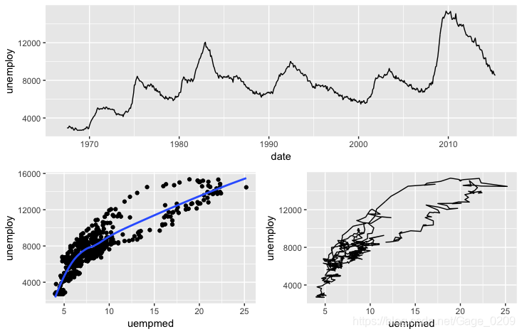
此外,除了ggplot2,R中使用函数par()或layout()也可以容易的将多个图形组合为一副总图,具体参考《R语言实战》3.5图形的组合部分,这里不再赘述
本文来自互联网用户投稿,文章观点仅代表作者本人,不代表本站立场,不承担相关法律责任。如若转载,请注明出处。 如若内容造成侵权/违法违规/事实不符,请点击【内容举报】进行投诉反馈!