动手学习深度学习 09:循环神经网络
文章目录
- 01 序列模型
- 1、统计工具
- 2、自回归模型
- 2.1 马尔科夫假设
- 2.2 潜变量模型
- 3、训练
- 3.1 数据生成
- 3.2 模型搭建
- 3.3 训练模型
- 3.4 预测
- 02 文本预处理
- 1、读取数据集
- 2、词元化(分词)
- 3、词典
- 4、整合所有功能
- 5、小结
- 03 语言模型和数据集
- 1、语言模型
- 2、马尔可夫模型与n元语法
- 3、自然语言统计
- 4、读取长序列数据
- 4.1 随机采样
- 4.2 顺序分区
- 04 循环神经网络(RNN)
- 1、RNN
- 2、困惑度
- 3、梯度裁剪
- 05 RNN从零开始实现
- 06 RNN简洁实现
- 07 通过时间反向传播
01 序列模型
之前的图片数据都是空间信息,而NLP的数据为时序结构的
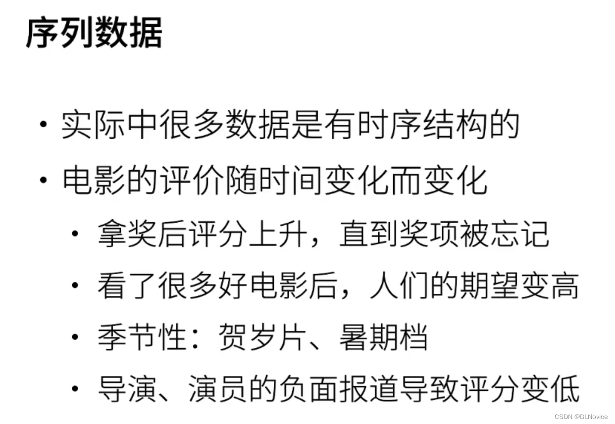
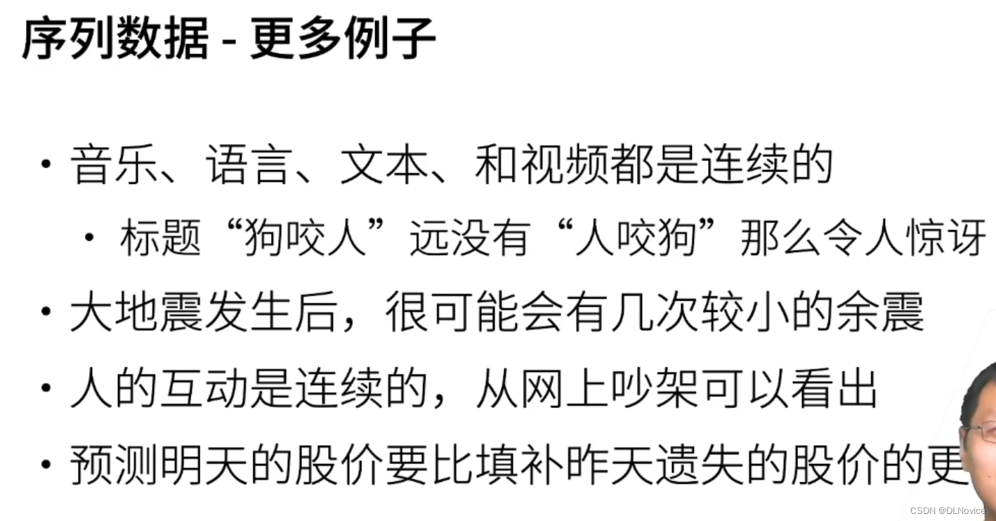
看一下更多有关序列数据的例子:
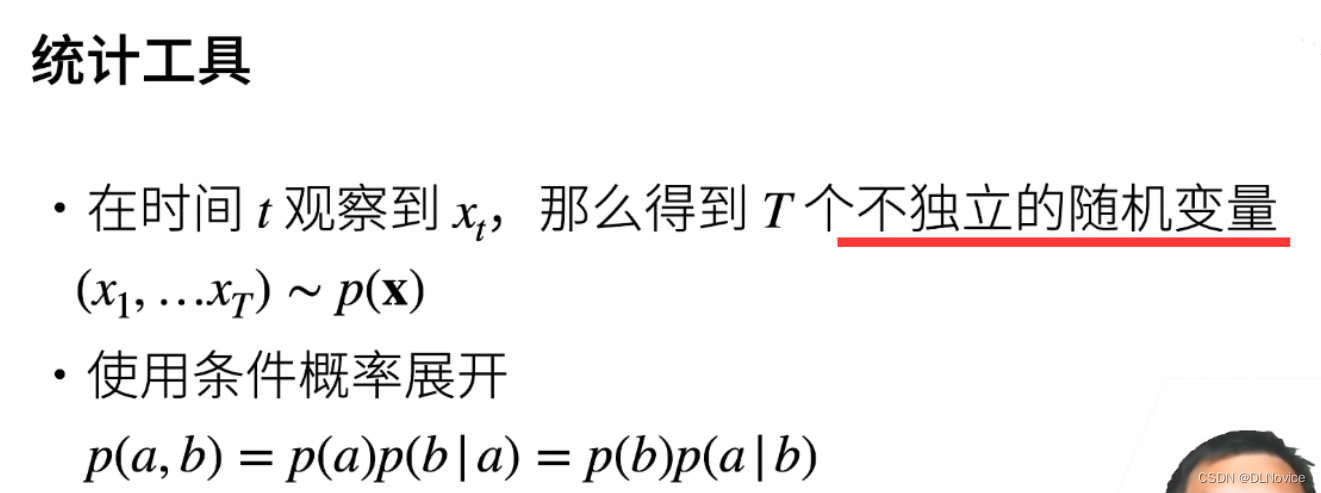
1、统计工具
如何对数据进行建模:
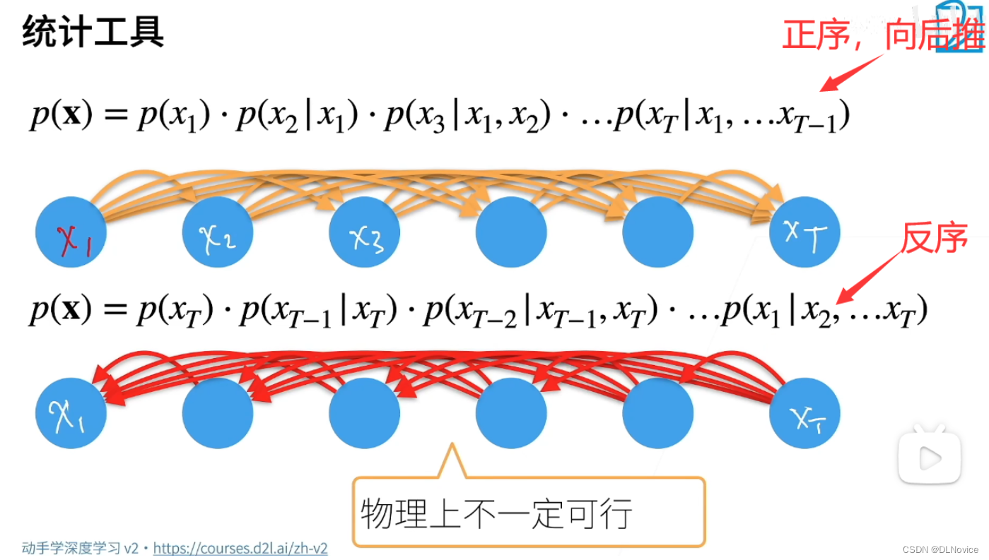
反序是有一定意义的,根据未来事件推理之前的事件,虽然物理上不一定可行,但是对于rnn来说,正反都可以。
2、自回归模型
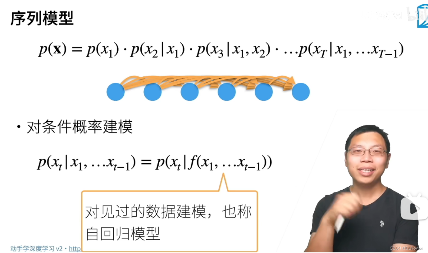
下面我们详细阐述两个方案:
2.1 马尔科夫假设
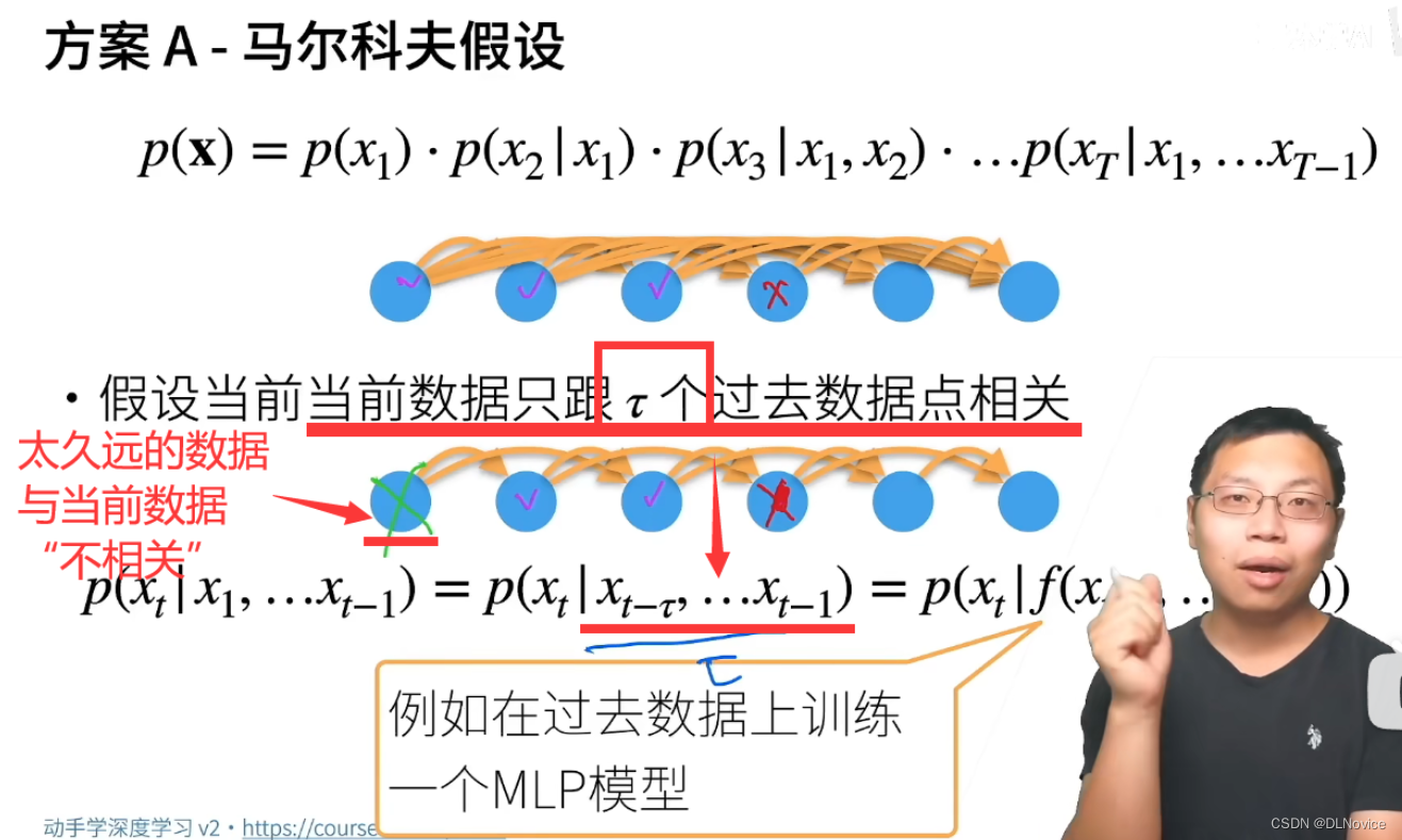
比如股票,跟一周前相关、跟一个月前相关、跟一年相关,但跟10年前关系可能就不大了
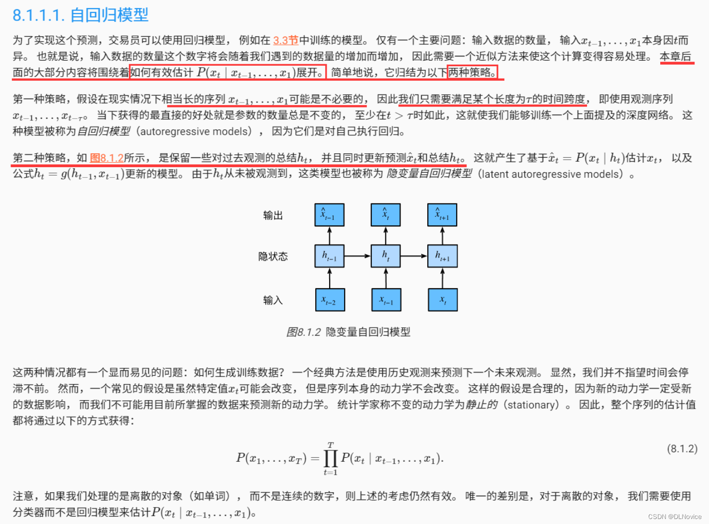
2.2 潜变量模型
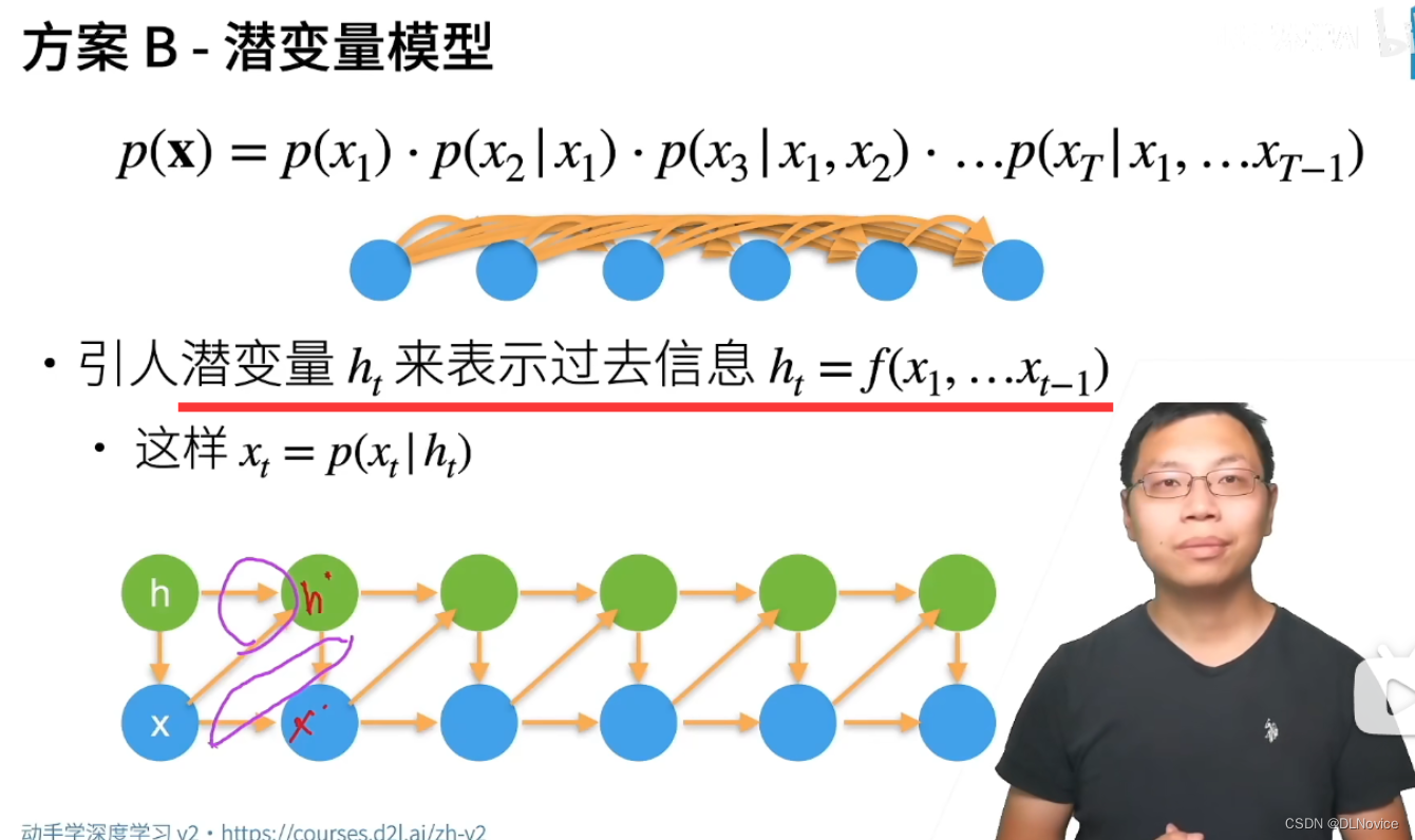
总结
- 时序模型中,当前数据跟之前观察到的数据相关
- 自回归模型使用自身过去数据来预测未来
- 马尔科夫模型假设当前只跟最近少数数据相关,从而简化模型
- 潜变量模型使用潜变量来概括历史信息
3、训练
3.1 数据生成
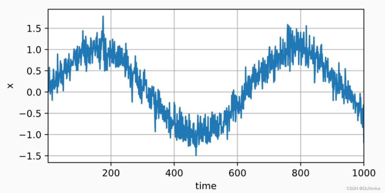
使用正弦函数和一些可加性噪声来生成序列数据, 时间步为1,2,…,1000。
%matplotlib inline
import torch
from torch import nn
from d2l import torch as d2lT = 1000  # 总共产生1000个点
time = torch.arange(1, T + 1, dtype=torch.float32)
x = torch.sin(0.01 * time) + torch.normal(0, 0.2, (T,))
d2l.plot(time, [x], 'time', 'x', xlim=[1, 1000], figsize=(6, 3))
结果展示:
3.2 模型搭建
基于马尔可夫假设训练nlp模型:

tau = 4
features = torch.zeros((T - tau, tau))  # (样本数,特征数)
for i in range(tau):features[:, i] = x[i: T - tau + i]
labels = x[tau:].reshape((-1, 1))batch_size, n_train = 16, 600
# 只有前n_train个样本用于训练
train_iter = d2l.load_array((features[:n_train], labels[:n_train]),batch_size, is_train=True)
使用一个相当简单的架构训练模型: 一个拥有两个全连接层的多层感知机,ReLU激活函数和平方损失。
# 初始化网络权重的函数
def init_weights(m):if type(m) == nn.Linear:nn.init.xavier_uniform_(m.weight)# 一个简单的多层感知机
def get_net():net = nn.Sequential(nn.Linear(4, 10),nn.ReLU(),nn.Linear(10, 1))net.apply(init_weights)return net# 平方损失。注意:MSELoss计算平方误差时不带系数1/2
loss = nn.MSELoss(reduction='none')
3.3 训练模型
def train(net, train_iter, loss, epochs, lr):trainer = torch.optim.Adam(net.parameters(), lr)for epoch in range(epochs):for X, y in train_iter:trainer.zero_grad()l = loss(net(X), y)l.sum().backward()trainer.step()print(f'epoch {epoch + 1}, 'f'loss: {d2l.evaluate_loss(net, train_iter, loss):f}')net = get_net()
train(net, train_iter, loss, 5, 0.01)
epoch 1, loss: 0.069569
epoch 2, loss: 0.055816
epoch 3, loss: 0.053317
epoch 4, loss: 0.051390
epoch 5, loss: 0.050837
3.4 预测
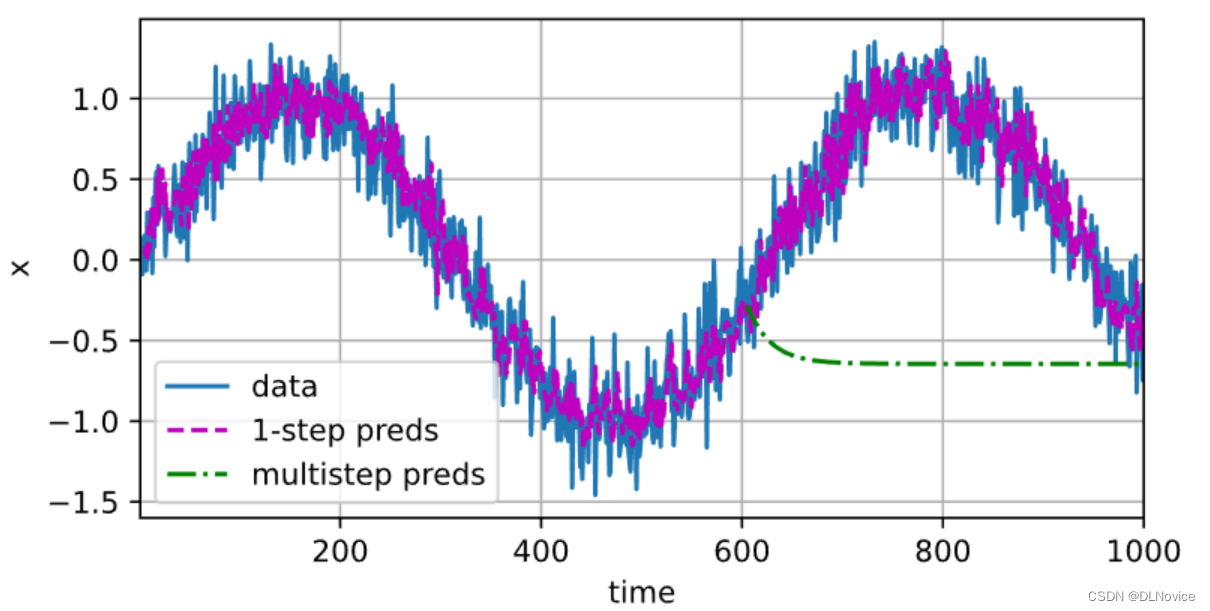
由于训练损失很小,因此我们期望模型能有很好的工作效果。 让我们看看这在实践中意味着什么。 首先是检查模型预测下一个时间步的能力, 也就是单步预测(one-step-ahead prediction)。
onestep_preds = net(features)
d2l.plot([time, time[tau:]],[x.detach().numpy(), onestep_preds.detach().numpy()], 'time','x', legend=['data', '1-step preds'], xlim=[1, 1000],figsize=(6, 3))
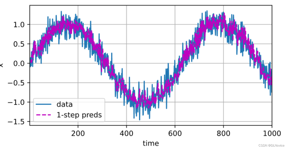
可以看到预测的大体趋势和真实数据差不多。
我们做这种预测是比较容易的,已知4个数据,预测下一个,然后又知道4个数据,再预测下一个,难的情况是,基于你预测的结果再去预测下一步,这样误差会累计,我们预测股票不是只预测一天两天,也需要长远的预测。
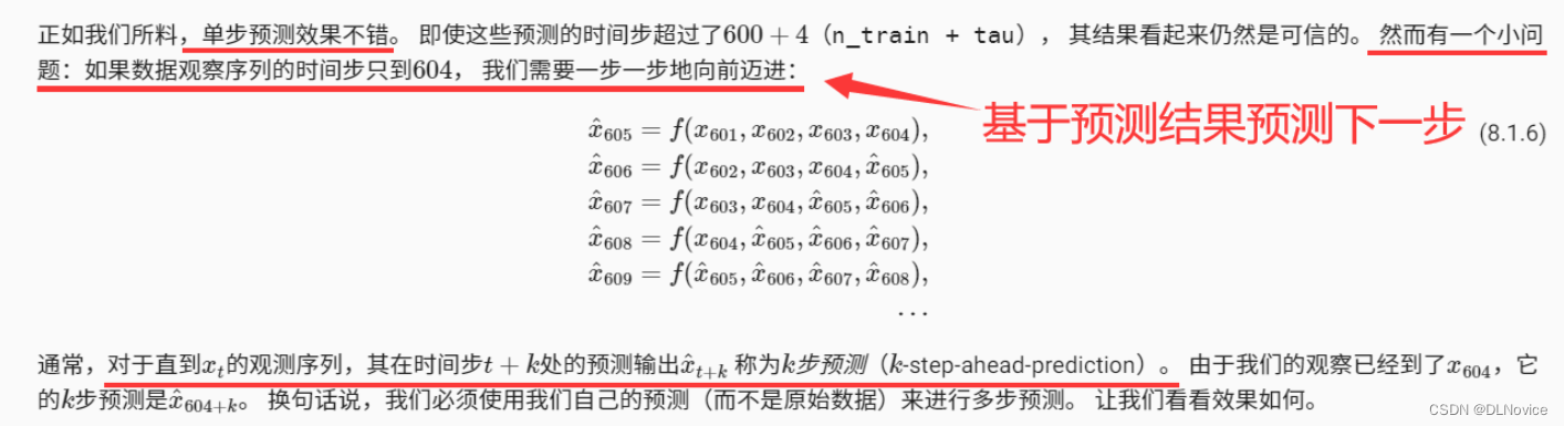
下面我们不采用单步预测了,用k步预测,你会看到预测结果逐渐离谱。
multistep_preds = torch.zeros(T)
multistep_preds[: n_train + tau] = x[: n_train + tau]
for i in range(n_train + tau, T):multistep_preds[i] = net(multistep_preds[i - tau:i].reshape((1, -1)))d2l.plot([time, time[tau:], time[n_train + tau:]],[x.detach().numpy(), onestep_preds.detach().numpy(),multistep_preds[n_train + tau:].detach().numpy()], 'time','x', legend=['data', '1-step preds', 'multistep preds'],xlim=[1, 1000], figsize=(6, 3))
效果展示:
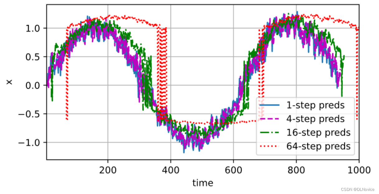
基于k=1,4,16,64,通过对整个序列预测的计算, 让我们更仔细地看一下k步预测的困难。
max_steps = 64features = torch.zeros((T - tau - max_steps + 1, tau + max_steps))
# 列i(i
for i in range(tau):features[:, i] = x[i: i + T - tau - max_steps + 1]# 列i(i>=tau)是来自(i-tau+1)步的预测,其时间步从(i)到(i+T-tau-max_steps+1)
for i in range(tau, tau + max_steps):features[:, i] = net(features[:, i - tau:i]).reshape(-1)steps = (1, 4, 16, 64)
d2l.plot([time[tau + i - 1: T - max_steps + i] for i in steps],[features[:, (tau + i - 1)].detach().numpy() for i in steps], 'time', 'x',legend=[f'{i}-step preds' for i in steps], xlim=[5, 1000],figsize=(6, 3))
02 文本预处理
对于序列数据处理问题,我们在 8.1节中 评估了所需的统计工具和预测时面临的挑战。 这样的数据存在许多种形式,文本是最常见例子之一。
本节中,我们将解析文本的常见预处理步骤。 这些步骤通常包括:
- 将文本作为字符串加载到内存中。
- 将字符串拆分为词元(如单词和字符)。
- 建立一个词表,将拆分的词元映射到数字索引。
- 将文本转换为数字索引序列,方便模型操作。
import collections
import re
from d2l import torch as d2l
1、读取数据集
#@save
d2l.DATA_HUB['time_machine'] = (d2l.DATA_URL + 'timemachine.txt','090b5e7e70c295757f55df93cb0a180b9691891a')def read_time_machine():  #@save"""将时间机器数据集加载到文本行的列表中"""with open(d2l.download('time_machine'), 'r') as f:lines = f.readlines()return [re.sub('[^A-Za-z]+', ' ', line).strip().lower() for line in lines]lines = read_time_machine()
print(f'# 文本总行数: {len(lines)}')
print(lines[0])
print(lines[10])
Downloading ..\data\timemachine.txt from http://d2l-data.s3-accelerate.amazonaws.com/timemachine.txt...
# 文本总行数: 3221
the time machine by h g wells
twinkled and his usually pale face was flushed and animated the
2、词元化(分词)
下面的tokenize函数将文本行列表(lines)作为输入, 列表中的每个元素是一个文本序列(如一条文本行),返回一个由词元列表组成的列表,其中的每个词元都是一个字符串(string)。
def tokenize(lines, token='word'):  #@save"""将文本行拆分为单词或字符词元"""if token == 'word':return [line.split() for line in lines]elif token == 'char':return [list(line) for line in lines]else:print('错误:未知词元类型:' + token)tokens = tokenize(lines)
for i in range(11):print(tokens[i])
输出展示:
['the', 'time', 'machine', 'by', 'h', 'g', 'wells']
[]
[]
[]
[]
['i']
[]
[]
['the', 'time', 'traveller', 'for', 'so', 'it', 'will', 'be', 'convenient', 'to', 'speak', 'of', 'him']
['was', 'expounding', 'a', 'recondite', 'matter', 'to', 'us', 'his', 'grey', 'eyes', 'shone', 'and']
['twinkled', 'and', 'his', 'usually', 'pale', 'face', 'was', 'flushed', 'and', 'animated', 'the']
3、词典
词元的类型是字符串,而模型需要的输入是数字,因此这种类型不方便模型使用。 现在,让我们构建一个字典,通常也叫做词表(vocabulary), 用来将字符串类型的词元映射到从0开始的数字索引中。
- 我们先将训练集中的所有文档合并在一起,对它们的唯一词元进行统计, 得到的统计结果称之为语料(corpus)。
- 然后根据每个唯一词元的出现频率,为其分配一个数字索引。 很少出现的词元通常被移除,这可以降低复杂性。
- 另外,语料库中不存在或已删除的任何词元都将映射到一个特定的未知词元“”。
- 我们可以选择增加一个列表,用于保存那些被保留的词元, 例如:填充词元(“”); 序列开始词元(“”); 序列结束词元(“”)。
class Vocab: #@save"""文本词表"""def __init__(self, tokens=None, min_freq=0, reserved_tokens=None):if tokens is None:tokens = []if reserved_tokens is None:reserved_tokens = []# 按出现频率排序counter = count_corpus(tokens)self._token_freqs = sorted(counter.items(), key=lambda x: x[1],reverse=True)# 未知词元的索引为0self.idx_to_token = ['' ] + reserved_tokensself.token_to_idx = {token: idxfor idx, token in enumerate(self.idx_to_token)}for token, freq in self._token_freqs:if freq < min_freq:breakif token not in self.token_to_idx:self.idx_to_token.append(token)self.token_to_idx[token] = len(self.idx_to_token) - 1def __len__(self):return len(self.idx_to_token)def __getitem__(self, tokens):if not isinstance(tokens, (list, tuple)):return self.token_to_idx.get(tokens, self.unk)return [self.__getitem__(token) for token in tokens]def to_tokens(self, indices):if not isinstance(indices, (list, tuple)):return self.idx_to_token[indices]return [self.idx_to_token[index] for index in indices]@propertydef unk(self): # 未知词元的索引为0return 0@propertydef token_freqs(self):return self._token_freqsdef count_corpus(tokens): #@save"""统计词元的频率"""# 这里的tokens是1D列表或2D列表if len(tokens) == 0 or isinstance(tokens[0], list):# 将词元列表展平成一个列表tokens = [token for line in tokens for token in line]return collections.Counter(tokens)
我们首先使用时光机器数据集作为语料库来构建词表,然后打印前几个高频词元及其索引。
vocab = Vocab(tokens)
print(list(vocab.token_to_idx.items())[:10])
[('' , 0), ('the', 1), ('i', 2), ('and', 3), ('of', 4), ('a', 5), ('to', 6), ('was', 7), ('in', 8), ('that', 9)]
现在,我们可以将每一条文本行转换成一个数字索引列表。
for i in [0, 10]:print('文本:', tokens[i])print('索引:', vocab[tokens[i]])
文本: ['the', 'time', 'machine', 'by', 'h', 'g', 'wells']
索引: [1, 19, 50, 40, 2183, 2184, 400]
文本: ['twinkled', 'and', 'his', 'usually', 'pale', 'face', 'was', 'flushed', 'and', 'animated', 'the']
索引: [2186, 3, 25, 1044, 362, 113, 7, 1421, 3, 1045, 1]
4、整合所有功能
在使用上述函数时,我们将所有功能打包到load_corpus_time_machine函数中, 该函数返回corpus(词元索引列表)和vocab(时光机器语料库的词表)。
为了简化后面章节中的训练,我们使用字符(而不是单词)实现文本词元化
def load_corpus_time_machine(max_tokens=-1):  #@save"""返回时光机器数据集的词元索引列表和词表"""lines = read_time_machine()tokens = tokenize(lines, 'char')vocab = Vocab(tokens)# 因为时光机器数据集中的每个文本行不一定是一个句子或一个段落,# 所以将所有文本行展平到一个列表中corpus = [vocab[token] for line in tokens for token in line]if max_tokens > 0:corpus = corpus[:max_tokens]return corpus, vocabcorpus, vocab = load_corpus_time_machine()
len(corpus), len(vocab)
(170580, 28)
5、小结
- 文本是序列数据的一种最常见的形式之一。
- 为了对文本进行预处理,我们通常将文本拆分为词元,构建词表将词元字符串映射为数字索引,并将文本数据转换为词元索引以供模型操作。
03 语言模型和数据集
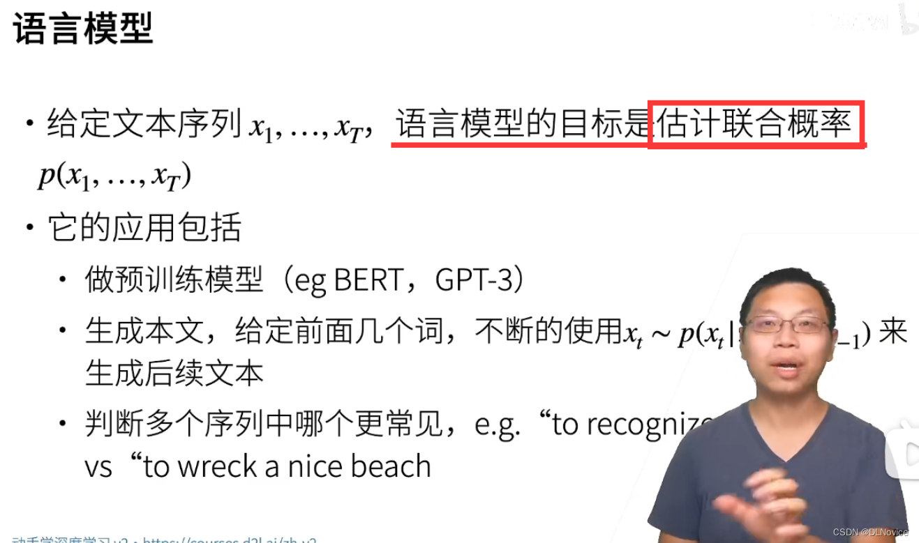
1、语言模型
2、马尔可夫模型与n元语法
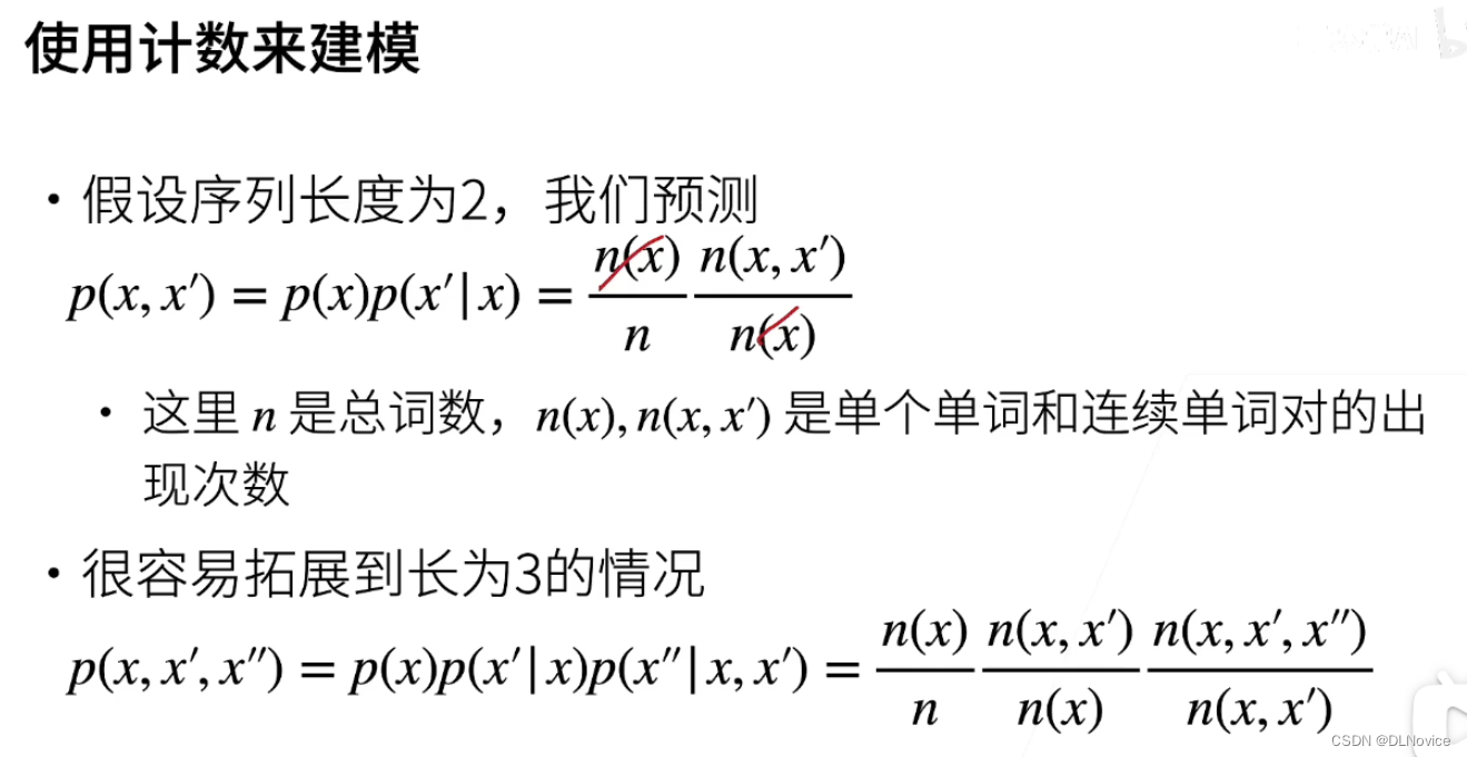
但如果序列很长怎么办?
使用马尔科夫假设,降低复杂度
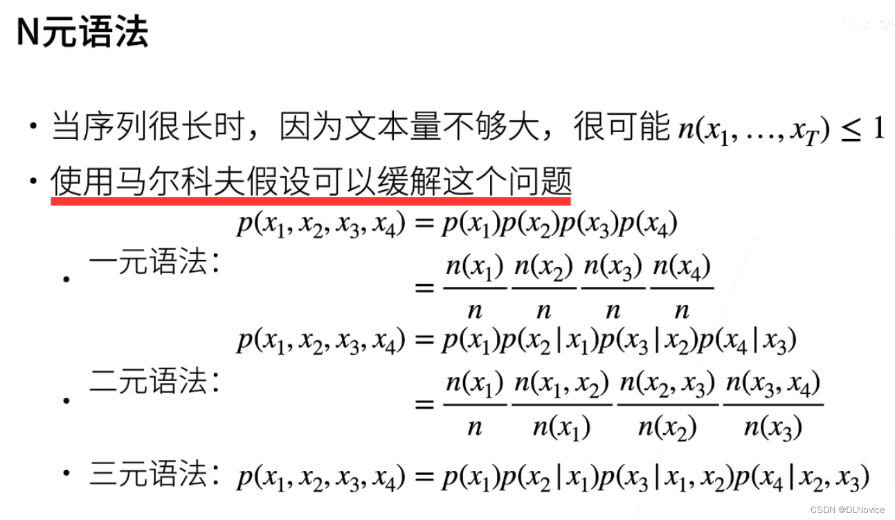
通常,涉及一个、两个和三个变量的概率公式分别被称为 “一元语法”(unigram)、“二元语法”(bigram)和“三元语法”(trigram)模型。 下面,我们将学习如何去设计更好的模型。
总结:
- 语言模型估计文本序列的联合概率
- 使用统计方法时常采用n元语法
3、自然语言统计
根据 8.2节中介绍的时光机器数据集构建词表, 并打印前10个最常用的(频率最高的)单词。
import random
import torch
from d2l import torch as d2ltokens = d2l.tokenize(d2l.read_time_machine())
# 因为每个文本行不一定是一个句子或一个段落,因此我们把所有文本行拼接到一起
corpus = [token for line in tokens for token in line]
vocab = d2l.Vocab(corpus)
vocab.token_freqs[:10]
结果展示:
[('the', 2261),('i', 1267),('and', 1245),('of', 1155),('a', 816),('to', 695),('was', 552),('in', 541),('that', 443),('my', 440)]
最流行的词看起来很无聊, 这些词通常被称为停用词(stop words),可以被过滤掉。
还有个明显的问题是词频衰减的速度相当地快。 例如,最常用单词的词频对比,第10个还不到第1个的1/5。 为了更好地理解,我们可以画出的词频图:
freqs = [freq for token, freq in vocab.token_freqs]
d2l.plot(freqs, xlabel='token: x', ylabel='frequency: n(x)',xscale='log', yscale='log')
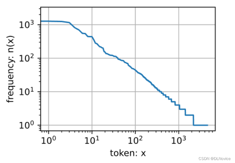
像极了我们常说的一句话:80%的财富掌握在20%的人手里。
其他次元组合,如二元语法、三元语法等等,又会是如何呢?
bigram_tokens = [pair for pair in zip(corpus[:-1], corpus[1:])]
bigram_vocab = d2l.Vocab(bigram_tokens)
bigram_vocab.token_freqs[:10]
[(('of', 'the'), 309),(('in', 'the'), 169),(('i', 'had'), 130),(('i', 'was'), 112),(('and', 'the'), 109),(('the', 'time'), 102),(('it', 'was'), 99),(('to', 'the'), 85),(('as', 'i'), 78),(('of', 'a'), 73)]
这里值得注意:在十个最频繁的词对中,有九个是由两个停用词组成的, 只有一个与“the time”有关。 我们再进一步看看三元语法的频率是否表现出相同的行为方式。
trigram_tokens = [triple for triple in zip(corpus[:-2], corpus[1:-1], corpus[2:])]
trigram_vocab = d2l.Vocab(trigram_tokens)
trigram_vocab.token_freqs[:10]
[(('the', 'time', 'traveller'), 59),(('the', 'time', 'machine'), 30),(('the', 'medical', 'man'), 24),(('it', 'seemed', 'to'), 16),(('it', 'was', 'a'), 15),(('here', 'and', 'there'), 15),(('seemed', 'to', 'me'), 14),(('i', 'did', 'not'), 14),(('i', 'saw', 'the'), 13),(('i', 'began', 'to'), 13)]
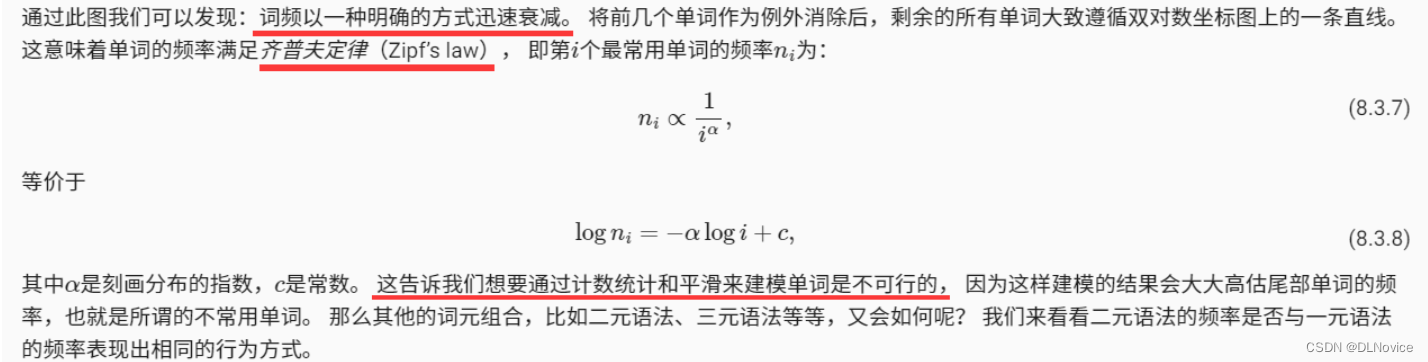
最后,我们直观地对比三种模型中的词元频率:一元语法、二元语法和三元语法。
bigram_freqs = [freq for token, freq in bigram_vocab.token_freqs]
trigram_freqs = [freq for token, freq in trigram_vocab.token_freqs]
d2l.plot([freqs, bigram_freqs, trigram_freqs], xlabel='token: x',ylabel='frequency: n(x)', xscale='log', yscale='log',legend=['unigram', 'bigram', 'trigram'])
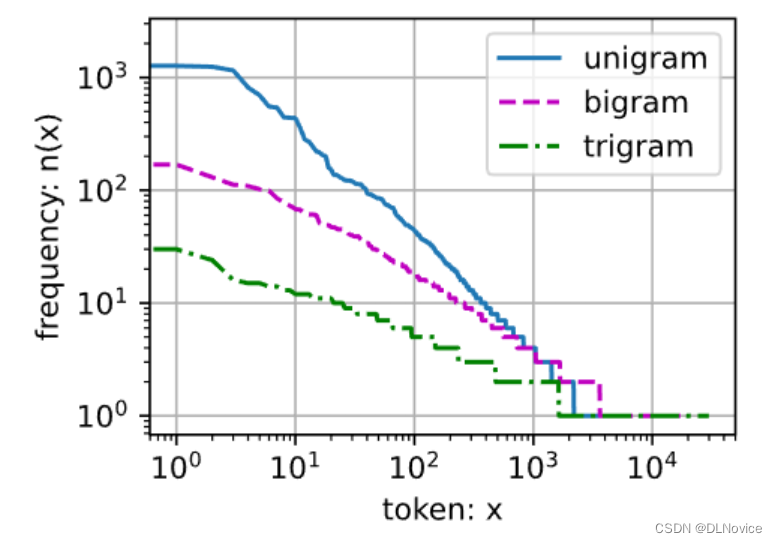
这张图非常令人振奋!原因有很多:
- 首先,除了一元语法词,单词序列似乎也遵循齐普夫定律, 尽管公式 (8.3.7)中的指数α更小 (指数的大小受序列长度的影响)。
- 其次,词表中n元组的数量并没有那么大,这说明语言中存在相当多的结构, 这些结构给了我们应用模型的希望。
- 第三,很多n元组很少出现,这使得拉普拉斯平滑非常不适合语言建模。
作为代替,我们将使用基于深度学习的模型。
4、读取长序列数据
下面我们来聊一个重要的话题。
由于序列数据本质上是连续的,因此我们在处理数据时需要解决这个问题。 在 8.1节中我们以一种相当特别的方式做到了这一点: 当序列变得太长而不能被模型一次性全部处理时, 我们可能希望拆分这样的序列方便模型读取。
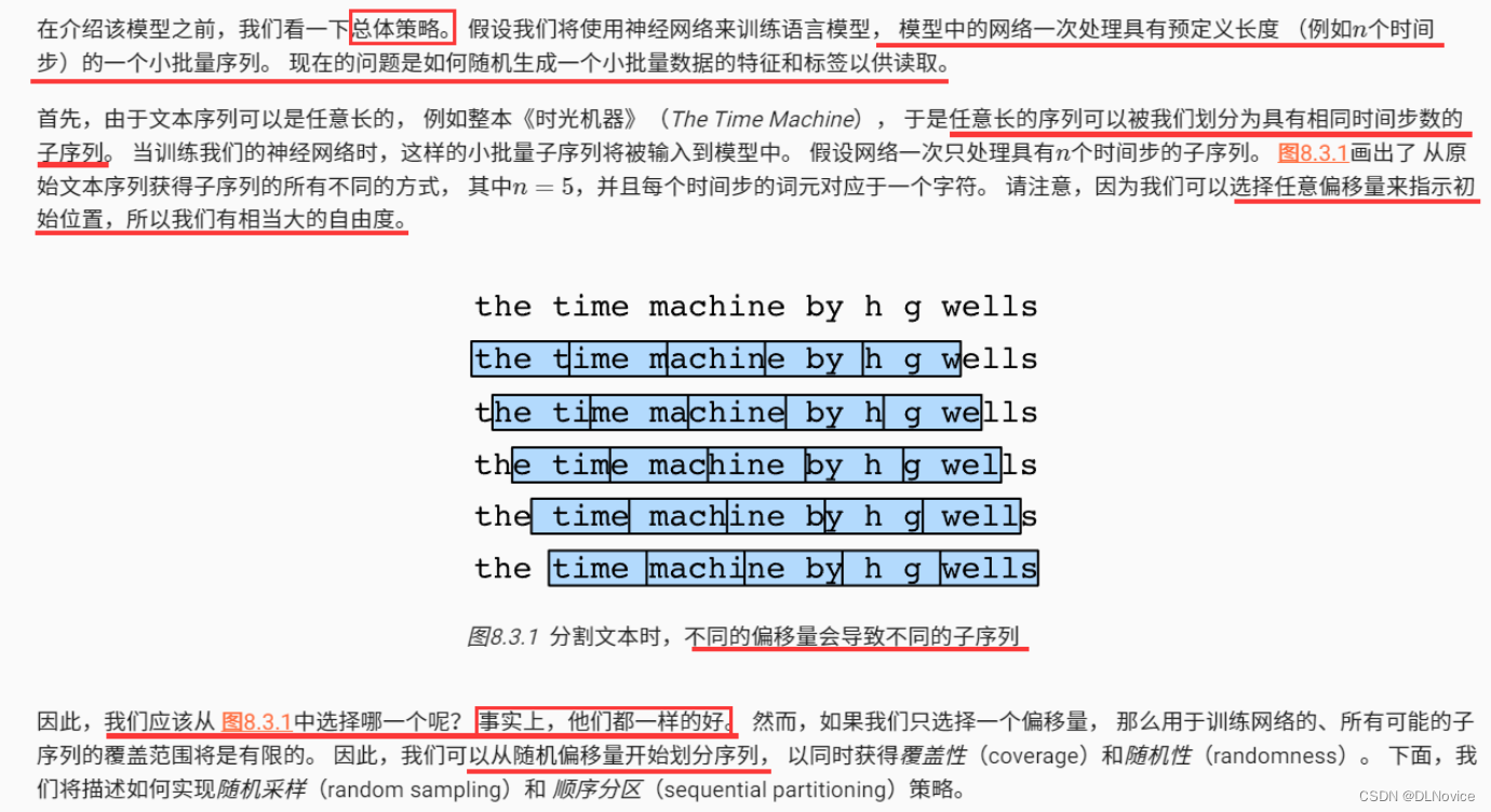
下面,我们将描述如何实现随机采样(random sampling)和 顺序分区(sequential partitioning)策略。
4.1 随机采样
在随机采样中,每个样本都是在原始的长序列上任意捕获的子序列。 在迭代过程中,来自两个相邻的、随机的、小批量中的子序列不一定在原始序列上相邻。 对于语言建模,目标是基于到目前为止我们看到的词元来预测下一个词元, 因此标签是移位了一个词元的原始序列。
下面的代码每次可以从数据中随机生成一个小批量。 在这里,参数batch_size指定了每个小批量中子序列样本的数目, 参数num_steps是每个子序列中预定义的时间步数。
def seq_data_iter_random(corpus, batch_size, num_steps): #@save"""使用随机抽样生成一个小批量子序列"""# 从随机偏移量开始对序列进行分区,随机范围包括num_steps-1corpus = corpus[random.randint(0, num_steps - 1):]# 减去1,是因为我们需要考虑标签num_subseqs = (len(corpus) - 1) // num_steps# 长度为num_steps的子序列的起始索引initial_indices = list(range(0, num_subseqs * num_steps, num_steps))# 在随机抽样的迭代过程中,# 来自两个相邻的、随机的、小批量中的子序列不一定在原始序列上相邻random.shuffle(initial_indices)def data(pos):# 返回从pos位置开始的长度为num_steps的序列return corpus[pos: pos + num_steps]num_batches = num_subseqs // batch_sizefor i in range(0, batch_size * num_batches, batch_size):# 在这里,initial_indices包含子序列的随机起始索引initial_indices_per_batch = initial_indices[i: i + batch_size]X = [data(j) for j in initial_indices_per_batch]Y = [data(j + 1) for j in initial_indices_per_batch]yield torch.tensor(X), torch.tensor(Y)
下面我们生成一个从0到34的序列。 假设批量大小为2,时间步数为5,这意味着可以生成 ⌊(35−1)/5⌋=6个“特征-标签”子序列对。 如果设置小批量大小为2,我们只能得到3个小批量。
my_seq = list(range(35))
for X, Y in seq_data_iter_random(my_seq, batch_size=2, num_steps=5):print('X: ', X, '\nY:', Y)
X:  tensor([[14, 15, 16, 17, 18],[ 9, 10, 11, 12, 13]])
Y: tensor([[15, 16, 17, 18, 19],[10, 11, 12, 13, 14]])
X:  tensor([[19, 20, 21, 22, 23],[29, 30, 31, 32, 33]])
Y: tensor([[20, 21, 22, 23, 24],[30, 31, 32, 33, 34]])
X:  tensor([[ 4,  5,  6,  7,  8],[24, 25, 26, 27, 28]])
Y: tensor([[ 5,  6,  7,  8,  9],[25, 26, 27, 28, 29]])
4.2 顺序分区
在迭代过程中,除了对原始序列可以随机抽样外, 我们还可以保证两个相邻的小批量中的子序列在原始序列上也是相邻的。 这种策略在基于小批量的迭代过程中保留了拆分的子序列的顺序,因此称为顺序分区。
def seq_data_iter_sequential(corpus, batch_size, num_steps): #@save"""使用顺序分区生成一个小批量子序列"""# 从随机偏移量开始划分序列offset = random.randint(0, num_steps)num_tokens = ((len(corpus) - offset - 1) // batch_size) * batch_sizeXs = torch.tensor(corpus[offset: offset + num_tokens])Ys = torch.tensor(corpus[offset + 1: offset + 1 + num_tokens])Xs, Ys = Xs.reshape(batch_size, -1), Ys.reshape(batch_size, -1)num_batches = Xs.shape[1] // num_stepsfor i in range(0, num_steps * num_batches, num_steps):X = Xs[:, i: i + num_steps]Y = Ys[:, i: i + num_steps]yield X, Y
基于相同的设置,通过顺序分区读取每个小批量的子序列的特征X和标签Y。 通过将它们打印出来可以发现: 迭代期间来自两个相邻的小批量中的子序列在原始序列中确实是相邻的。
for X, Y in seq_data_iter_sequential(my_seq, batch_size=2, num_steps=5):print('X: ', X, '\nY:', Y)
X:  tensor([[ 4,  5,  6,  7,  8],[19, 20, 21, 22, 23]])
Y: tensor([[ 5,  6,  7,  8,  9],[20, 21, 22, 23, 24]])
X:  tensor([[ 9, 10, 11, 12, 13],[24, 25, 26, 27, 28]])
Y: tensor([[10, 11, 12, 13, 14],[25, 26, 27, 28, 29]])
X:  tensor([[14, 15, 16, 17, 18],[29, 30, 31, 32, 33]])
Y: tensor([[15, 16, 17, 18, 19],[30, 31, 32, 33, 34]])
现在,我们将上面的两个采样函数包装到一个类中, 以便稍后可以将其用作数据迭代器。
class SeqDataLoader: #@save"""加载序列数据的迭代器"""def __init__(self, batch_size, num_steps, use_random_iter, max_tokens):if use_random_iter:self.data_iter_fn = d2l.seq_data_iter_randomelse:self.data_iter_fn = d2l.seq_data_iter_sequentialself.corpus, self.vocab = d2l.load_corpus_time_machine(max_tokens)self.batch_size, self.num_steps = batch_size, num_stepsdef __iter__(self):return self.data_iter_fn(self.corpus, self.batch_size, self.num_steps)
最后,我们定义了一个函数load_data_time_machine, 它同时返回数据迭代器和词表, 因此可以与其他带有load_data前缀的函数 (如 3.5节中定义的 d2l.load_data_fashion_mnist)类似地使用。
def load_data_time_machine(batch_size, num_steps, #@saveuse_random_iter=False, max_tokens=10000):"""返回时光机器数据集的迭代器和词表"""data_iter = SeqDataLoader(batch_size, num_steps, use_random_iter, max_tokens)return data_iter, data_iter.vocab
小结:
- 语言模型是自然语言处理的关键。
- n元语法通过截断相关性,为处理长序列提供了一种实用的模型。
- 长序列存在一个问题:它们很少出现或者从不出现。
- 齐普夫定律支配着单词的分布,这个分布不仅适用于一元语法,还适用于其他n元语法。
- 通过拉普拉斯平滑法可以有效地处理结构丰富而频率不足的低频词词组。
- 读取长序列的主要方式是随机采样和顺序分区。在迭代过程中,后者可以保证来自两个相邻的小批量中的子序列在原始序列上也是相邻的。
04 循环神经网络(RNN)
1、RNN
首先我们回顾一下“潜变量自回归模型”

下面看一下怎么把这个模变成RNN:
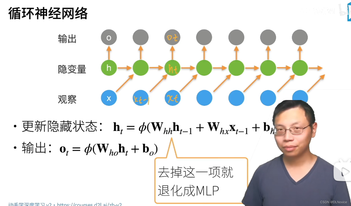
注意ot与xt-1、xt的关系,为了避免弄错,我们看一下下图:
- 对当前“观察”进行预测,得到输出
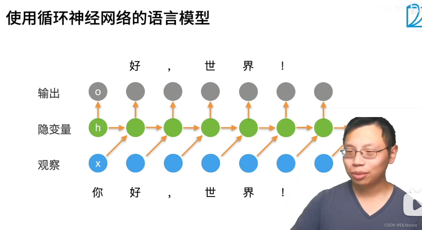
计算损失时是用ot与xt计算损失。
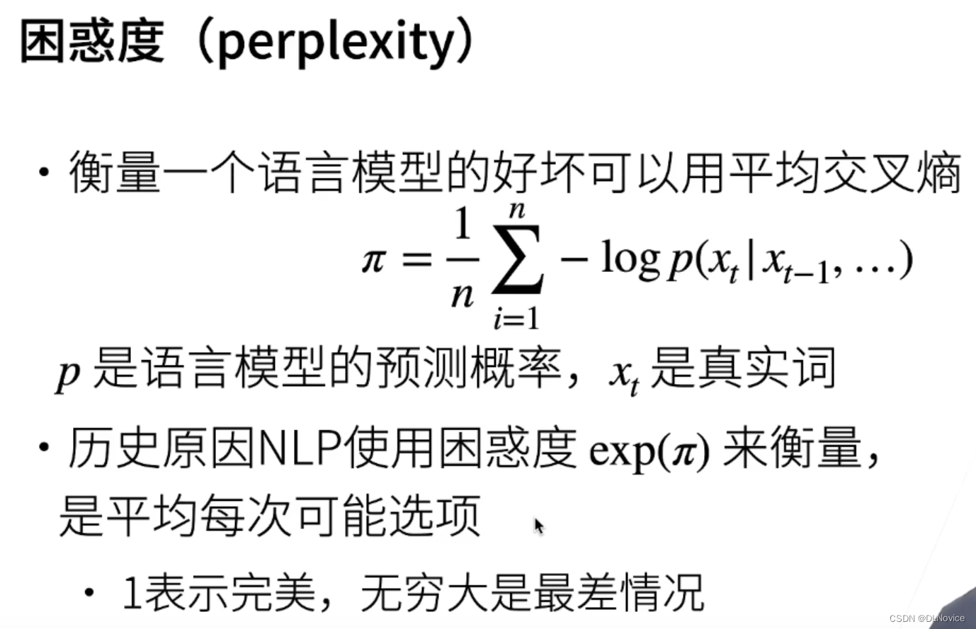
2、困惑度
如何衡量一个语言模型的好坏?困惑度
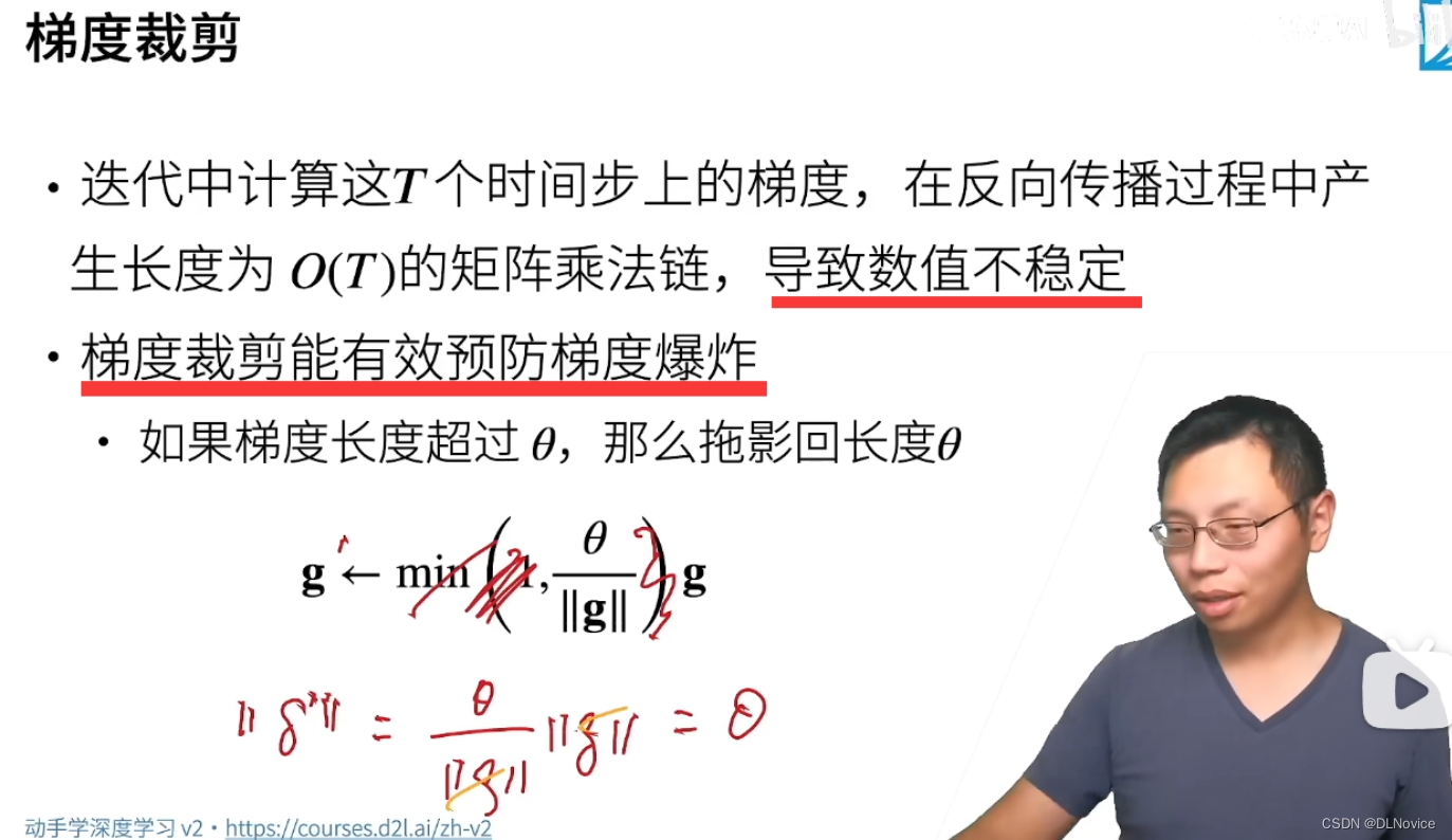
3、梯度裁剪
下面讲一个重要工具:梯度裁剪
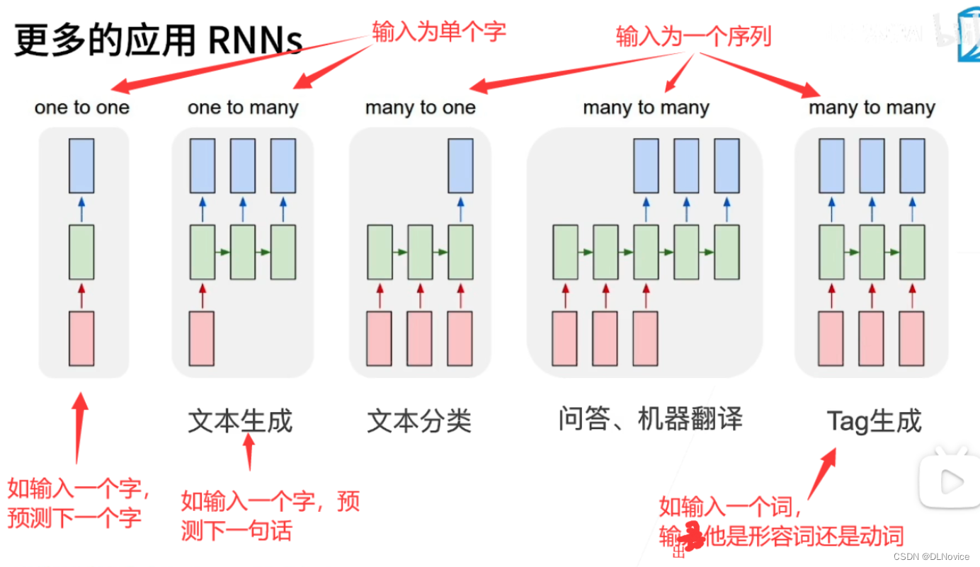
RNN的应用:
总结:
- 循环神经网络的输出取决于当下输入和前一个时间的隐变量
- 应用到语言模型时,循环神经网络根据当前词预测下一次时刻词
- 通常使用困惑度来衡量语言模型的好坏
05 RNN从零开始实现
- 8.5. 循环神经网络的从零开始实现 — 动手学深度学习 2.0.0-beta1 documentation (d2l.ai)
06 RNN简洁实现
- 8.6. 循环神经网络的简洁实现 — 动手学深度学习 2.0.0-beta1 documentation (d2l.ai)
07 通过时间反向传播
- 8.7. 通过时间反向传播 — 动手学深度学习 2.0.0-beta1 documentation (d2l.ai)
本文来自互联网用户投稿,文章观点仅代表作者本人,不代表本站立场,不承担相关法律责任。如若转载,请注明出处。 如若内容造成侵权/违法违规/事实不符,请点击【内容举报】进行投诉反馈!