立体匹配网络中的domain adaptation问题：AdaStereo

文章目录

• 概述
• 损失函数

概述

• 希望讨论的问题是什么？
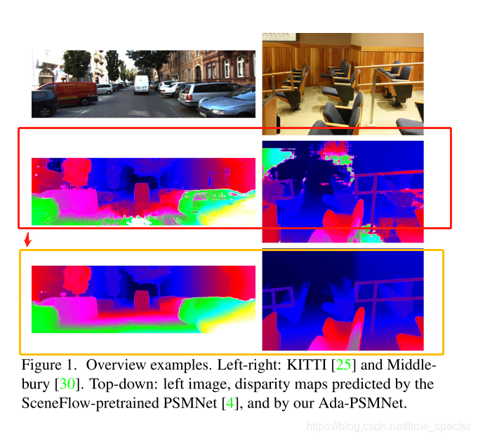
  以PSMNet为例，其在Middlebury数据集上进行预训练得到的模型，在KITTI上的推理效果或许就不好。这篇文章就想聊聊怎么去处理不同场景下的模型的适应问题。又或者说，模型的泛化问题。

• 参考论文及相关信息为：
  
  是商汤2020年的工作。

• 论文的效果怎么样？
  

• 能否简要概述是怎么解决的问题？
  假定现在有两个数据集，一个是合成数据集，数据量非常大，另一个是真实场景数据集，数据量相对小很多，文章认为这两个数据集之间的gap主要在于以下几个层面：

  1. input image

  1. “At the input image level, color and brightness are the obvious gaps.”
  2. 通过提出一个 non-adversarial progressive color transfer算法将输入的color space与target影像的场景进行对齐，这个过程通过网络训练完成。

  2. internal cost volume

  3. ‘…significant differences in distributions’
  4. 使用了cost normalization 层，用于配准cost distribution。主要使用了两个归一化操作：channel normalization以及pixel normalization

  3. output disparity

  5. ‘Moreover, geometries of the output disparity maps are inconsistent as well’
  6. self- supervised occlusion-aware reconstruction,

提出了AdaStereo，旨在构建一个标准的场景自适应网络，网络结构为：

已知：

1. 作为source的大量合成数据集 ( I s t , I s r ) (I_s^t,I_s^r) (Ist​,Isr​)
2. 合成数据集的真实视差 d s l ^ \hat{d_s^l} dsl​^​
3. 作为target的少量真实数据集 ( I t l , I t r ) (I_t^l,I_t^r) (Itl​,Itr​)

希望的推理输出：

1. 真实场景的视差 d t l d_t^l dtl​

损失函数

整体的损失函数为：
L = L s m a i n + λ s o c c L s o c c + λ t a r L t a r + λ t o c c L t o c c + λ t s m L t s m L=L_{s}^{m a i n}+\lambda_{s}^{o c c} L_{s}^{o c c}+\lambda_{t}^{a r} L_{t}^{a r}+\lambda_{t}^{o c c} L_{t}^{o c c}+\lambda_{t}^{s m} L_{t}^{s m} L=Lsmain​+λsocc​Lsocc​+λtar​Ltar​+λtocc​Ltocc​+λtsm​Ltsm​
其中的$\lambda$为对应的loss weights。

损失函数中的五项具体为：

1. source domain层面的视差回归loss：
   L s m a i n = S m o o t h L 1 ( d s l − d s l ^ ) L_s^{main} = Smooth_{L1}(d_s^l-\hat{d_s^l}) Lsmain​=SmoothL1​(dsl​−dsl​^​)

2. 在souce domain层面的occlusion mask训练损失，使用binary cross entropy loss：
   L s o c c = B C E ( O s l , O s l ^ ) L_s^{occ} = BCE(O_s^l,\hat{O_s^l}) Lsocc​=BCE(Osl​,Osl​^​)

3. 在target domain层面，the occlusion-aware appearance reconstruction loss：
   L t a r = α 1 − S S I M ( I t l ⊙ ( 1 − O t l ) , I t l ‾ ⊙ ( 1 − O t l ) ) 2 + ( 1 − α ) ∥ I t l ⊙ ( 1 − O t l ) − I t l ‾ ⊙ ( 1 − O t l ) ∥ 1 \begin{aligned} L_{t}^{a r}=& \alpha \frac{1-S S I M\left(I_{t}^{l} \odot\left(1-O_{t}^{l}\right), \overline{I_{t}^{l}} \odot\left(1-O_{t}^{l}\right)\right)}{2} \\ &+(1-\alpha)\left\|I_{t}^{l} \odot\left(1-O_{t}^{l}\right)-\overline{I_{t}^{l}} \odot\left(1-O_{t}^{l}\right)\right\|_{1} \end{aligned} Ltar​=​α21−SSIM(Itl​⊙(1−Otl​),Itl​​⊙(1−Otl​))​+(1−α)∥∥∥​Itl​⊙(1−Otl​)−Itl​​⊙(1−Otl​)∥∥∥​1​​

   其中，$\odot$表示逐元素的乘法，SSIM表示simplified single scale SSIM项（3*3的block filter），以及$\alpha$设置为0.85。

4. 在target domain中，在occulusion mask上使用$L1$正则项:
   L t o c c = ∣ ∣ O t l ∣ ∣ 1 L_t^{occ}=||O_t^l||_1 Ltocc​=∣∣Otl​∣∣1​

5. 在target-domain上，使用edge-aware项作为target-domain中的视差平滑项，其中$\partial$表示gradient,
   L t s m = ∣ ∂ x d t l ∣ e − ∣ ∂ x I t l ∣ + ∣ ∂ y d t l ∣ e − ∣ ∂ y I t l ∣ L_{t}^{s m}=\left|\partial_{x} d_{t}^{l}\right| e^{-\left|\partial_{x} I_{t}^{l}\right|}+\left|\partial_{y} d_{t}^{l}\right| e^{-\left|\partial_{y} I_{t}^{l}\right|} Ltsm​=∣∣​∂x​dtl​∣∣​e−∣∂x​Itl​∣+∣∣​∂y​dtl​∣∣​e−∣∂y​Itl​∣

本文来自互联网用户投稿，文章观点仅代表作者本人，不代表本站立场，不承担相关法律责任。如若转载，请注明出处。 如若内容造成侵权/违法违规/事实不符，请点击【内容举报】进行投诉反馈！