[QUANTAXIS量化分析]成长股内在价值投资策略

基本原理

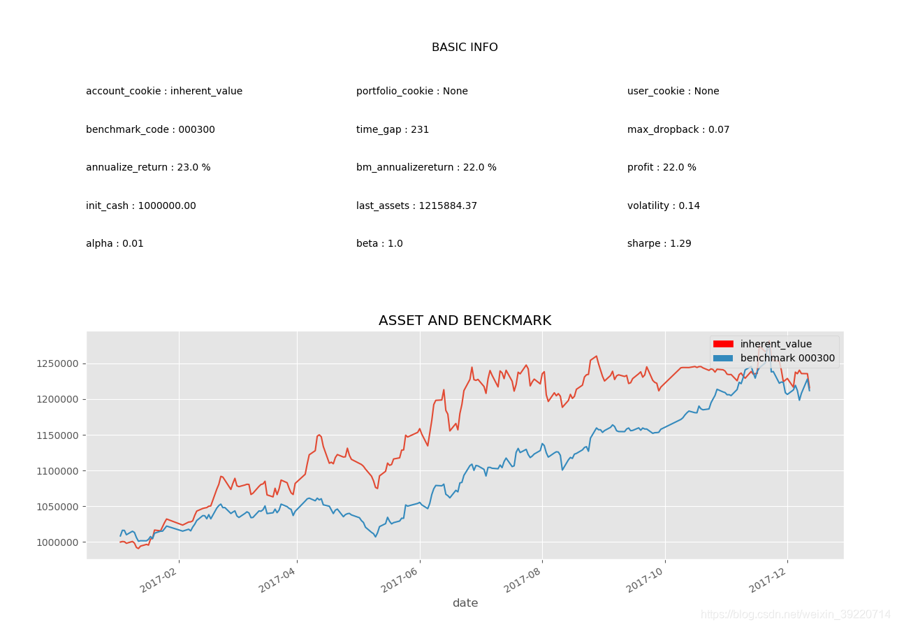
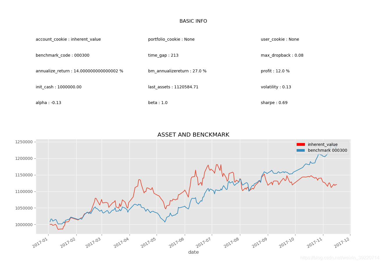
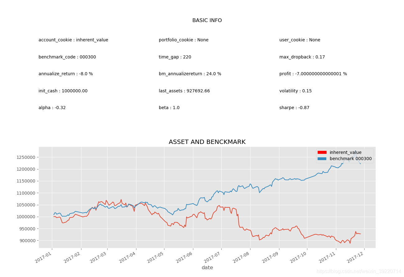
• 以一个十分简便的成长股估价公式计算出的数据，十分接近于一些更加复杂的数学计算所得出的结果
• 格雷厄姆成长股内在价值公式：
  
  Value = Current(Normal)Earnings * (8.5 plus twice the excepted annual growth rate)
• 可直接表示为：value = E * (8.5 + 2 * R)
• E 表示每股收益（ EPS） ，决定了公司内在价值的基准； R 表示预期收益增长率，体现了公司的未来盈利能力；数值 8.5 被格雷厄姆认为是一家预期收益增长率为 0 的公司的合理市盈率，故（ 8.5+2*R） 可以被视为预期收益增长率为 R 的公司的合理市盈率。股票每股收益和其合理市盈率的乘积则直观的给出了合理的估值水平。

策略实现

• 选取市盈率0-20的股票作为将要执行的股票，共332支
• 初始资金100万，时间段：2017-01-01~2018-01-01
• R 表示预期收益增长率，用线性回归拟合前n个EPS，得到EPS=a+bt，用b/整个回归时间区间的平均EPS近似为增长率
• 选取 Value/Price 在 1 到1.2 之间的股票进入组合。
• 最多持有十支股票，已持有的重复买入，每天排序一次
• 运行截图：
  
• 8.5 倍的市盈率对于 A 股市场普遍的高市盈率来说可能偏低，调整为9后的运行截图：
  
• 再调整为10：
  

代码如下

# coding: utf-8
# @author: lin
# @date: 2018/11/20import QUANTAXIS as QA
import pandas as pd
import time
import matplotlib.pyplot as plt
import numpy as np
from sklearn import linear_modelpd.set_option('max_colwidth', 5000)
pd.set_option('display.max_columns', 5000)
pd.set_option('display.max_rows', 5000)class InherentValue:def __init__(self, start_time, stop_time, n_stock=10, stock_init_cash=1000000, n_EPS_before=5):self.Account = QA.QA_Account()  # 初始化账户self.Account.reset_assets(stock_init_cash)  # 初始化账户self.Account.account_cookie = 'inherent_value'self.Broker = QA.QA_BacktestBroker()self.time_quantum_list = ['-12-31', '-09-30', '-06-30', '-03-31']self.start_time = start_timeself.stop_time = stop_timeself.n_EPS_before = n_EPS_beforeself.n_stock = n_stockself.stock_pool = []self.data = Noneself.ind = Noneself.get_stock_pool()def get_financial_time(self):"""得到此日期前一个财务数据的日期:return:"""year = self.start_time[0:4]while (True):for day in self.time_quantum_list:the_financial_time = year + dayif the_financial_time <= self.start_time:return the_financial_timeyear = str(int(year) - 1)def get_assets_eps(self, stock_code, the_financial_time):"""得到高级财务数据:param stock_code::param the_financial_time: 离开始时间最近的财务数据的时间:return:"""financial_report = QA.QA_fetch_financial_report(stock_code, the_financial_time)if financial_report is not None:return financial_report.iloc[0]['totalAssets'], financial_report.iloc[0]['EPS']return None, Nonedef get_stock_pool(self):"""选取哪些股票"""stock_code_list = QA.QA_fetch_stock_list_adv().code.tolist()the_financial_time = self.get_financial_time()for stock_code in stock_code_list:# print(stock_code)assets, EPS = self.get_assets_eps(stock_code, the_financial_time)if assets is not None and EPS != 0:data = QA.QA_fetch_stock_day_adv(stock_code, self.start_time, self.stop_time)if data is None:continueprice = data.to_pd().iloc[0]['close']if 0 < price / EPS < 20:  # 满足条件才添加进行排序# print(price / EPS)self.stock_pool.append(stock_code)def linear_model_main(self, x_parameters, y_parameters, predict_value):# Create linear regression objectregr = linear_model.LinearRegression()regr.fit(x_parameters, y_parameters)predict_outcome = regr.predict(predict_value)prediction = {}prediction['intercept'] = regr.intercept_prediction['coefficient'] = regr.coef_prediction['predicted_value'] = predict_outcomereturn predictiondef get_value(self, stock_code, the_time):# 由财政数据中得到EPS，是上个季度的# 对纯净EPS做线性回归，不用ln的原因是有负值时会出错year = the_time[0:4]if_break = Falsen_EPS_list = []while (True):for day in self.time_quantum_list:date = year + dayif date < the_time:financial_report = QA.QA_fetch_financial_report(stock_code, date)if financial_report is not None:n_EPS_list.append(financial_report.iloc[0]['EPS'])# n_EPS_list[date] = financial_report.iloc[0]['EPS']if len(n_EPS_list) >= self.n_EPS_before:  # 求几何平均值时需要一共n+1个数据if_break = Truebreakif if_break:  # 触发，则跳出循环breakyear = str(int(year) - 1)  # 今年没有财政数据则换成前一年time_list = [[self.n_EPS_before - i] for i in range(self.n_EPS_before)]# 一个做变量x，一个做变量yprediction = self.linear_model_main(time_list, n_EPS_list, self.n_EPS_before + 1)coefficient = prediction['coefficient']increase_ratio = coefficient / np.mean(n_EPS_list)value = n_EPS_list[0] * (9 + 2 * increase_ratio)         # 8.5可能过小，可以适当提高，试试效果如何return valuedef get_decided_para(self, data):# 将决定性因子作为决策点，可以购入则置为1data['decided_para'] = 0data['value_price'] = 0# data.drop(['open', 'high', 'low', 'volume', 'amount'], axis=1, inplace=True)if_first = Truelast_index = Nonefor index, row in data.iterrows():       # 事实证明可行，datastruct的add一个函数是对每一支单独计算的if_value_equal = True  # 值是否跟上次值相同the_time = str(index[0])[:10]if not if_first:last_time = str(last_index[0])[:10]for time_quantum in self.time_quantum_list:middle_time = last_time[:4] + time_quantum  # 得到判断的分界点if last_time < middle_time < the_time:  # 有一次处于分界点左右，则需要重新计算if_value_equal = Falsebreakif if_value_equal:data.loc[index, 'value_price'] = data.loc[last_index, 'value_price']data.loc[index, 'decided_para'] = data.loc[last_index, 'decided_para']if if_first or not if_value_equal:stock_code = str(index[1])# print(stock_code)value = self.get_value(stock_code, the_time)price = row['close']  # 价格用当天收盘价来表示data.loc[index, 'value_price'] = value / priceif 1 < (value / price) < 1.2:data.loc[index, 'decided_para'] = 1if_first = Falselast_index = index  # 把当次时间加入，下次调用则为上次时间return datadef solve_data(self):self.data = QA.QA_fetch_stock_day_adv(self.stock_pool, self.start_time, self.stop_time)self.ind = self.data.add_func(self.get_decided_para)def run(self):self.solve_data()for items in self.data.panel_gen:today_time = items.index[0][0]one_day_data = self.ind.loc[today_time]  # 得到有包含因子的DataFrameone_day_data['date'] = items.index[0][0]one_day_data.reset_index(inplace=True)one_day_data.sort_values(by=['decided_para', 'value_price'], axis=0, ascending=False, inplace=True)today_stock = list(one_day_data.iloc[0:self.n_stock]['code'])one_day_data.set_index(['date', 'code'], inplace=True)one_day_data = QA.QA_DataStruct_Stock_day(one_day_data)  # 转换格式，便于计算bought_stock_list = list(self.Account.hold.index)print("SELL:")for stock_code in bought_stock_list:# 如果直接在循环中对bought_stock_list操作，会跳过一些元素if stock_code not in today_stock:try:item = one_day_data.select_day(str(today_time)).select_code(stock_code)order = self.Account.send_order(code=stock_code,time=today_time,amount=self.Account.sell_available.get(stock_code, 0),towards=QA.ORDER_DIRECTION.SELL,price=0,order_model=QA.ORDER_MODEL.MARKET,amount_model=QA.AMOUNT_MODEL.BY_AMOUNT)self.Broker.receive_order(QA.QA_Event(order=order, market_data=item))trade_mes = self.Broker.query_orders(self.Account.account_cookie, 'filled')res = trade_mes.loc[order.account_cookie, order.realorder_id]order.trade(res.trade_id, res.trade_price, res.trade_amount, res.trade_time)except Exception as e:print(e)print('BUY:')for stock_code in today_stock:try:item = one_day_data.select_day(str(today_time)).select_code(stock_code)if item.to_json()[0]['decided_para'] == 1:        # 可购买order = self.Account.send_order(code=stock_code,time=today_time,amount=1000,towards=QA.ORDER_DIRECTION.BUY,price=0,order_model=QA.ORDER_MODEL.CLOSE,amount_model=QA.AMOUNT_MODEL.BY_AMOUNT)self.Broker.receive_order(QA.QA_Event(order=order, market_data=item))trade_mes = self.Broker.query_orders(self.Account.account_cookie, 'filled')res = trade_mes.loc[order.account_cookie, order.realorder_id]order.trade(res.trade_id, res.trade_price, res.trade_amount, res.trade_time)except Exception as e:print(e)self.Account.settle()Risk = QA.QA_Risk(self.Account)print(Risk.message)# plt.show()Risk.assets.plot()  # 总资产plt.show()Risk.benchmark_assets.plot()  # 基准收益的资产plt.show()Risk.plot_assets_curve()  # 两个合起来的对比图plt.show()Risk.plot_dailyhold()  # 每只股票每天的买入量plt.show()start = time.time()
sss = InherentValue('2017-01-01', '2018-01-01')
stop = time.time()
print(stop - start)
print(len(sss.stock_pool))
sss.run()
stop2 = time.time()
print(stop2 - stop)

本文来自互联网用户投稿，文章观点仅代表作者本人，不代表本站立场，不承担相关法律责任。如若转载，请注明出处。 如若内容造成侵权/违法违规/事实不符，请点击【内容举报】进行投诉反馈！