使用 LSSVM 的 Matlab 演示求解反常微分方程问题（Matlab代码实现）

💥💥💞💞欢迎来到本博客❤️❤️💥💥

🏆博主优势：🌞🌞🌞博客内容尽量做到思维缜密，逻辑清晰，为了方便读者。

⛳️座右铭：行百里者，半于九十。

📋📋📋本文目录如下：🎁🎁🎁

目录

💥1 概述

📚2 运行结果

🎉3 参考文献

🌈4 Matlab代码实现

---

💥1 概述

LSSVM的特性

  1) 同样是对原始对偶问题进行求解，但是通过求解一个线性方程组（优化目标中的线性约束导致的）来代替SVM中的QP问题（简化求解过程），对于高维输入空间中的分类以及回归任务同样适用；

  2) 实质上是求解线性矩阵方程的过程，与高斯过程（Gaussian processes），正则化网络（regularization networks）和费雪判别分析（Fisher discriminant analysis）的核版本相结合；

  3) 使用了稀疏近似（用来克服使用该算法时的弊端）与稳健回归（稳健统计）；

  4) 使用了贝叶斯推断（Bayesian inference）；

  5) 可以拓展到非监督学习中：核主成分分析（kernel PCA）或密度聚类；

  6) 可以拓展到递归神经网络中。

📚2 运行结果

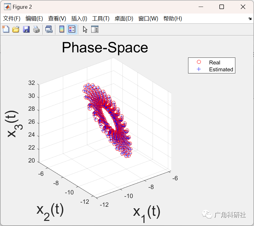
主函数部分代码：

% dot(x1)  = a * (x_2 -x_1)

% dot(x_2) = x_1 * (b- x_3) - x_2

% dot(x_3) = x_1 * x_2 -c* x_3

% 0 <=  t  < = t_f

% Initial Condition

% x_1(0) = -9.42, x_2(0)= -9.34, x_3(0)=28.3

% Theta=[a, b, c] = [10, 28, 8/3]

clear all; close all; clc

t0=0;

tf=10;

sampling_time=0.05;

t=(t0:sampling_time:tf)';

initial=[-9.42 -9.34 28.3]; % initial values of the ODE used for generating simulated data

ExactTheta=[10; 28 ; 8/3];  % The exact parameters of the lorenz system used for generating simulated data

cprintf( [1 0.1 0],'**** Excat parameters of the Lorenz system ***** \n\n');

fprintf('True theta_1= %f \n', ExactTheta(1));

fprintf('True theta_2= %f \n', ExactTheta(2));

fprintf('True theta_3= %f \n\n', ExactTheta(3));

fprintf( '************************************* \n\n');

%%  ========= Generating the simulation data ======================

options = odeset('RelTol',1e-5,'AbsTol',[1e-5 1e-5 1e-5]);

sol = ode45(@ridg,[t0 tf],initial,options,ExactTheta);

Y=deval(sol,t);

Y=Y';noise_level=0.01; % 0.03, 0.05, 0.07, 0.1

noise=noise_level*randn(size(t,1),1);

y1=Y(:,1)+noise;

y2=Y(:,2)+noise;

y3=Y(:,3)+noise;

🎉3 参考文献

部分理论来源于网络，如有侵权请联系删除。

[1]姜星宇. 基于动态粒子群算法的DPSO-LSSVM模型在短期电力负荷预测中的应用研究[D].沈阳农业大学,2022.DOI:10.27327/d.cnki.gshnu.2022.000596.

🌈4 Matlab代码实现

本文来自互联网用户投稿，文章观点仅代表作者本人，不代表本站立场，不承担相关法律责任。如若转载，请注明出处。 如若内容造成侵权/违法违规/事实不符，请点击【内容举报】进行投诉反馈！