NLP-Beginner 任务一:基于机器学习的文本分类(超详细!!)
NLP-Beginner 任务一:基于机器学习的文本分类
- 传送门
- 一. 介绍
- 1.1 任务简介
- 1.2 数据集
- 1.3 流程介绍
- 二. 特征提取
- 2.1 词袋特征(Bag-of-word)
- 2.2 N元特征 (N-gram)
- 三. 最优化求解
- 3.1 Softmax回归介绍
- 3.2 损失函数
- 3.3 梯度下降
- 3.4 学习率
- 四. 代码及实现
- 4.1 实验设置
- 4.2 结果展示
- 4.2.1 实验一
- 4.2.2 实验二
- 4.3 代码
- 4.3.1 主文件——main.py
- 4.3.2 特征提取——feature.py
- 4.3.3 Softmax回归——mysoftmax_regression.py
- 4.3.4 结果&画图——comparison_plot.py
- 五. 总结
- 六. 自我推销
传送门
NLP-Beginner 任务传送门
我的代码传送门
数据集传送门
一. 介绍
1.1 任务简介
本次的NLP(Natural Language Processing)任务是利用机器学习中的softmax回归(softmax regression)来对文本的情感进行分类。
1.2 数据集
数据集传送门
训练集共有15万余项,语言为英文,情感分为0~4共五种情感。
例子:
输入: A series of escapades demonstrating the adage that what is good for the goose is also good for the gander , some of which occasionally amuses but none of which amounts to much of a story .
输出: 1
输入: This quiet , introspective and entertaining independent is worth seeking .
输出: 4
输入:Even fans of Ismail Merchant 's work
输出: 2
输入: A positively thrilling combination of ethnography and all the intrigue , betrayal , deceit and murder of a Shakespearean tragedy or a juicy soap opera .
输出: 3
1.3 流程介绍
本篇博客将会一步一步讲解如何完成本次的NLP任务,具体流程为:
数据输入(英文句子)→特征提取(数字化数据)→最优化求解(求解softmax回归模型)→结果输出(情感类别)
二. 特征提取
2.1 词袋特征(Bag-of-word)
词袋模型即把句子拆解成一个一个单词,存在于句子的单词 (不区分大小写),则对应的向量位置上的数字为1,反之为0,通过这种方式,可以把一个句子变成一个由数字表示的0-1向量。
例子
单词:i, you, him, her, love, hate, but
句子A:I love you
向量a:[1,1,0,0,1,0,0]
句子B:I hate you
向量b:[1,1,0,0,0,1,0]
句子C:I love you but hate him
向量c:[1,1,1,0,1,1,1]
句子D:I hate you but love him
向量d:[1,1,1,0,1,1,1]
这种转换方式非常的简单,但是它没有考虑词序,比如句子C和句子D,两个意思完全不一样的句子对应的向量居然是完全一样的。因此,词袋模型在这种情况下会存在比较大的缺陷。
2.2 N元特征 (N-gram)
N元特征相较于词袋模型,则考虑了词序。
N元特征与词袋模型最大的不同就是,词袋模型仅考虑了单词存在与否,而N元特征考虑了词组存在与否。例如,当N=2时,I love you 不再看作是 I, love, you 这三个单词,而是 I love, love you 这两个词组。
通常来说,使用N元特征时,会一并使用1, 2, …, N-1元特征。
例子
特征(N=1&2):i, you, him, her, love, hate, but, i-love, i-hate, love-you, hate-you, you-but, but-love, but-hate, love-him, hate-him
句子A:I love you
向量a:[1,1,0,0,1,0,0,0,1,0,1,0,0,0,0,0,0]
句子B:I hate you
向量b:[1,1,0,0,0,1,0,1,0,1,0,1,0,0,0,0,0]
句子C:I love you but hate him
向量c:[1,1,1,0,1,1,1,1,1,0,1,0,1,0,1,0,1]
句子D:I hate you but love him
向量d:[1,1,1,0,1,1,1,1,0,1,0,1,1,1,0,1,0]
这种转换方式较为复杂,但是考虑了句子中的词序。还有需要值得注意的是,即使是N=2时,也会产生一些几乎不具有真实语义的词组,比如C中的you-but,它在现实场景中没有具体的语义,但是这些无意义的词组也有可能在分类中起到很关键的作用。
另一方面,随着N的递增,文本的特征数也会上涨,因此遇到数据量大的输入时,较大的N会导致结果模型训练极度缓慢。
三. 最优化求解
3.1 Softmax回归介绍
Softmax 回归详尽介绍——章节3.3
在Softmax回归中,给定一个输入x,输出一个y向量,y的长度即为类别的个数,总和为1,y中的数字是各类别的概率。
例如:(0~4共五类)
y = ( 0 , 0 , 0.7 , 0.25 , 0.05 ) T y=(0,0,0.7,0.25,0.05)^T y=(0,0,0.7,0.25,0.05)T
则代表,输入x,其是类别2的概率为0.7,类别3的概率为0.25,类别4的概率为0.05。
给定C个类别,
y ∈ { 1 , 2 , . . . , C } y \in \{1,2,...,C\} y∈{1,2,...,C}
具体公式为:
p ( y = c ∣ x ) = softmax ( w c T x ) = exp ( w c T x ) ∑ c ′ = 1 C exp ( w c T x ) p(y=c|x)=\text{softmax}(w^T_cx)=\frac{\exp{(w^T_cx)}}{\sum_{c'=1}^C\exp{(w^T_cx)}} p(y=c∣x)=softmax(wcTx)=∑c′=1Cexp(wcTx)exp(wcTx)
其中 w c w_c wc是第 c c c类的权重向量,记 W = [ w 1 , w 2 , . . . , w C ] W=[w_1,w_2,...,w_C] W=[w1,w2,...,wC]为权重矩阵,则上述公式可以表示为列向量:
y ^ = f ( x ) = softmax ( W T x ) = exp ( W T x ) 1 ⃗ c T exp ( W T x ) \widehat{y}=f(x)=\text{softmax}(W^Tx)=\frac{\exp{(W^Tx)}}{\vec{1}_c^T\exp{(W^Tx)}} y =f(x)=softmax(WTx)=1cTexp(WTx)exp(WTx)
y ^ \widehat{y} y 的每一个元素,代表对应类别的概率。
因此,接下来的步骤便是求解参数矩阵 W W W。
3.2 损失函数
有了模型,我们就要对模型的好坏做出一个评价。也就是说,给定一个参数矩阵 W W W,我们要去量化一个模型的好坏,那么我们就要定义一个损失函数。
一般来说,有以下几种损失函数:
| 函数 | 公式 | 注释 |
|---|---|---|
| 0-1损失函数 | I ( y ≠ f ( x ) ) I(y\ne f(x)) I(y=f(x)) | 不可导 |
| 绝对值损失函数 | | y − f ( x ) y-f(x) y−f(x)| | 适用于连续值 |
| 平方值损失函数 | ( y − f ( x ) ) 2 (y-f(x))^2 (y−f(x))2 | 适用于连续值 |
| 交叉熵损失函数 | − ∑ c y c log f c ( x ) -\sum_c y_c\log{f_c(x)} −∑cyclogfc(x) | 适用于分类 |
| 指数损失函数 | exp ( − y f ( x ) ) \exp(-yf(x)) exp(−yf(x)) | 适用于二分类 |
| 合页损失函数 | max ( 0 , 1 − y f ( x ) ) \text{max}(0,1-yf(x)) max(0,1−yf(x)) | 适用于二分类 |
因此,总上述表来看,我们应该使用交叉熵损失函数。
对于每一个样本n,其损失值为
L ( f W ( x ( n ) ) , y ( n ) ) = − ∑ c = 1 C y c ( n ) log y ^ c ( n ) = − ( y ( n ) ) T log y ^ ( n ) = − ( y ( n ) ) T log ( exp ( W T x ( n ) ) 1 ⃗ c T exp ( W T x ( n ) ) ) L(f_W(x^{(n)}),y^{(n)})=-\sum_{c=1}^C y_c^{(n)}\log{\widehat{y}_c^{(n)}}=-(y^{(n)})^T\log{\widehat{y}^{(n)}}=-(y^{(n)})^T\log\bigg(\frac{\exp{(W^Tx^{(n)})}}{\vec{1}_c^T\exp{(W^Tx^{(n)})}}\bigg) L(fW(x(n)),y(n))=−c=1∑Cyc(n)logy c(n)=−(y(n))Tlogy (n)=−(y(n))Tlog(1cTexp(WTx(n))exp(WTx(n)))
其中 y ( n ) = ( I ( c = 0 ) , I ( c = 2 ) , . . . , I ( c = C ) ) T y^{(n)}=\big(I(c=0),I(c=2),...,I(c=C)\big)^T y(n)=(I(c=0),I(c=2),...,I(c=C))T,是一个one-hot向量,即只有一个元素是1,其他全是0的向量。
注:下标 c c c 代表向量中的第 c c c 个元素,这里 C = 4 C=4 C=4 。
例子:
句子 x ( n ) x^{(n)} x(n) 的类别是第0类,则 y ( n ) = [ 1 , 0 , 0 , 0 , 0 ] T y^{(n)}=[1,0,0,0,0]^T y(n)=[1,0,0,0,0]T
而对于总体样本,总的损失值则是每个样本损失值的平均,即
L ( W ) = L W ( f W ( x ) , y ) = 1 N ∑ n = 1 N L W ( f W ( x ( n ) ) , y ( n ) ) L(W)=L_W(f_W(x),y)=\frac{1}{N}\sum_{n=1}^NL_W(f_W(x^{(n)}),y^{(n)}) L(W)=LW(fW(x),y)=N1n=1∑NLW(fW(x(n)),y(n))
有了损失函数,我们就可以通过找到损失函数的最小值,来求解最优的参数矩阵 W W W。
3.3 梯度下降
梯度下降的基本思想是,对于每个固定的参数,求其梯度(导数),然后利用梯度(导数),进行对参数的更新。
在这里,我们的梯度是
∂ L ( W ) ∂ W = − 1 N ∑ n = 1 N x ( n ) ( y ( n ) − y ^ W ( n ) ) T \frac{\partial L(W)}{\partial W}=-\frac{1}{N}\sum_{n=1}^Nx^{(n)}(y^{(n)}-\widehat{y}^{(n)}_W)^T ∂W∂L(W)=−N1n=1∑Nx(n)(y(n)−y W(n))T
具体求导过程比较复杂,可以参考Softmax 回归详尽介绍——章节3.3,这里直接当作结论使用。
梯度下降的公式是
W t + 1 ← W t − α ∂ L ( W t ) ∂ W t W_{t+1}\leftarrow W_t-\alpha \frac{\partial L(W_t)}{\partial W_t} Wt+1←Wt−α∂Wt∂L(Wt)
其中 α \alpha α为学习率。
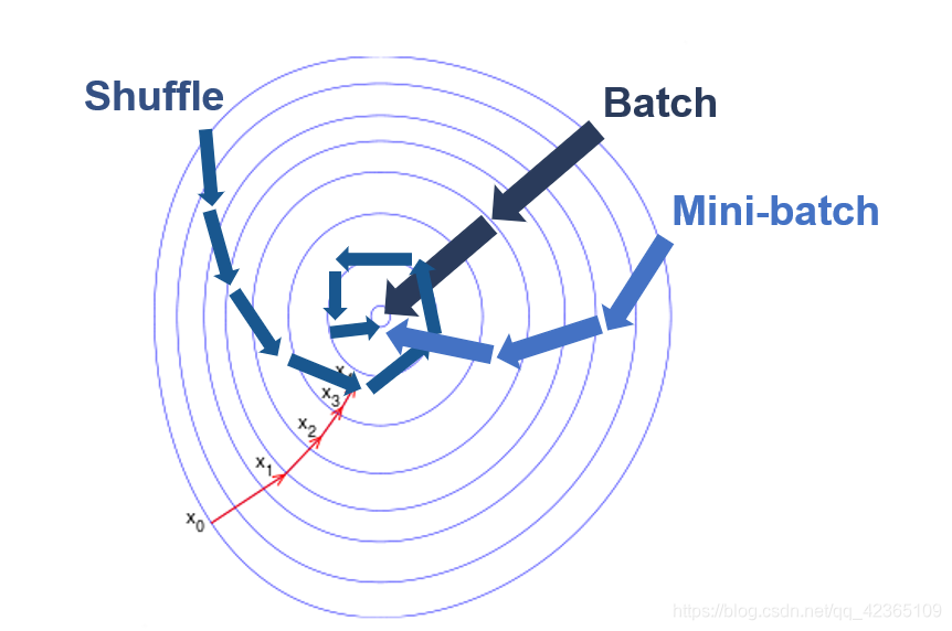
这种梯度下降的方式为最普通的梯度下降法——整批量梯度下降(Batch)。
还有另外两种梯度下降法:随机梯度下降(Shuffle),小批量梯度下降(Mini-Batch)。
随机梯度下降(Shuffle)
每次只随机取一个样本,即
Δ W = − x ( n ) ( y ( n ) − y ^ W ( n ) ) T \Delta W=-x^{(n)}(y^{(n)}-\widehat{y}^{(n)}_W)^T ΔW=−x(n)(y(n)−y W(n))T
然后直接进行更新
W t + 1 ← W t − α ( − Δ W t ) W_{t+1}\leftarrow W_t-\alpha(-\Delta W_t) Wt+1←Wt−α(−ΔWt)
小批量梯度下降(Mini-Batch)
每次随机取一些样本(如K个,样本集合为 S S S),即
Δ W = − 1 K ∑ n ∈ S x ( n ) ( y ( n ) − y ^ W ( n ) ) T \Delta W=-\frac{1}{K}\sum_{n\in S}x^{(n)}(y^{(n)}-\widehat{y}^{(n)}_W)^T ΔW=−K1n∈S∑x(n)(y(n)−y W(n))T
然后直接进行更新
W t + 1 ← W t − α ( − Δ W t ) W_{t+1}\leftarrow W_t-\alpha(-\Delta W_t) Wt+1←Wt−α(−ΔWt)
三种方法各有优缺点,见下表
| 方法 | 注释 |
|---|---|
| Batch | 优点:梯度准确 ; 缺点:每次计算复杂度为 O ( N ) O(N) O(N),时间开销大 |
| Shuffle | 优点:每次计算简单 ; 缺点: 梯度估计可能不准确,仅用到了一个样本 |
| Mini-Batch | 综合了Batch和Shuffle的策略,梯度较为准确,计算时间复杂度也较低 |
三种方法的简略示意图:
3.4 学习率
学习率相当于是步长。
小的步长使梯度下降缓慢,可能需要很久才到达最优点。
而大的步长虽然可能使函数“一步到位”降到最优值(最小值)附近,但是有可能会使函数在最小值附近剧烈震荡,导致不收敛,更严重地可能会使函数“跳”到一个较差的局部最小值,甚至越跳越远,永不收敛。
因此选取一个合适的学习率非常重要。
四. 代码及实现
4.1 实验设置
- 样本个数:1000
- 训练集:测试集 : 7:3
- 学习率:10-3~104
- Mini-Batch 大小:样本的1%
注意:为了看清这三种梯度下降的优劣,我们需要控制每种梯度下降的计算梯度的次数一致。
例如,假设样本量为1000,那么Batch循环一次就需要计算1000次梯度,而Shuffle循环一次只需要计算1次梯度,Mini-Batch循环一次需要计算1%*1000=10次梯度。
显然,如果规定相同的循环次数,那么肯定对Shuffle和Mini-Batch不公平,因此需要规定相同的计算梯度的次数。
例如,总次数为10000,样本量为1000,Batch就只能循环10000/1000=10次,Shuffle能循环10000/1=10000次,Mini-Batch能循环10000/(1%*1000)=1000次。
4.2 结果展示
4.2.1 实验一
首先进行计算梯度次数总数为10000的实验,结果如下图:
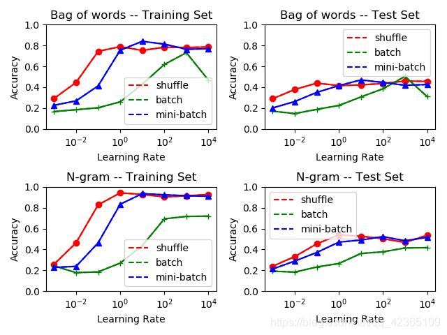
我们首先看向训练集。
对于不同的特征,我们可以看到N元特征明显要优于词袋模型,这是因为N元特征考虑了词序。
对于不同的学习率,我们可以看到,小的学习率并未让模型收敛,而大的学习率相比之下会更好。在本次实验中,并未出现大的学习率导致函数值震荡的现象。
对于不同的梯度下降,除了在学习率比较小不收敛的时,小批量和随机梯度下降表现几乎是相当的,而整批量梯度下降表现最差。
接着看向测试集,情况和训练集差不多。
基于以上的分析,我们可以得出以下结论:使用N元特征以及小批量(或随机)梯度下降,并且学习率设置为1左右,对于本数据集的Softmax回归模型参数求解效果最优。
4.2.2 实验二
接着进行计算梯度次数总数为100000的实验来看模型参数是否收敛,结果如下图:
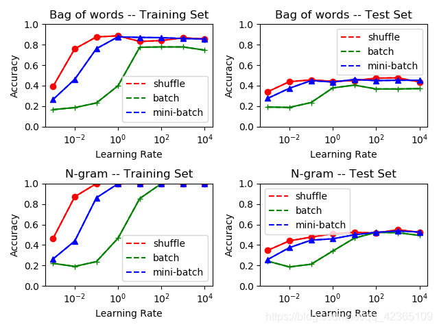
首先,结果和实验一的结论吻合,训练集的准确率高达100%,但这意味着其实模型存在着过拟合现象;而且,无论是实验一还是实验二,测试集的最高准确率都在55%附近,这意味着后面的90000次梯度计算只是在令模型过拟合,并未对模型的泛用性产生提升效果。
因此,尽管训练集的准确率看起来令人满意,但是过多的梯度下降只会使模型过拟合而不带来任何文本分类效果提升。
4.3 代码
4.3.1 主文件——main.py
import numpy
import csv
import random
from feature import Bag,Gram
from comparison_plot import alpha_gradient_plot# 数据读取
with open('train.tsv') as f:tsvreader = csv.reader(f, delimiter='\t')temp = list(tsvreader)# 初始化
data = temp[1:]
max_item=1000
random.seed(2021)
numpy.random.seed(2021)# 特征提取
bag=Bag(data,max_item)
bag.get_words()
bag.get_matrix()gram=Gram(data, dimension=2, max_item=max_item)
gram.get_words()
gram.get_matrix()# 画图
alpha_gradient_plot(bag,gram,10000,10)  # 计算10000次
alpha_gradient_plot(bag,gram,100000,10)  # 计算100000次
4.3.2 特征提取——feature.py
import numpy
import randomdef data_split(data, test_rate=0.3, max_item=1000):"""把数据按一定比例划分成训练集和测试集"""train = list()test = list()i = 0for datum in data:i += 1if random.random() > test_rate:train.append(datum)else:test.append(datum)if i > max_item:breakreturn train, testclass Bag:"""Bag of words"""def __init__(self, my_data, max_item=1000):self.data = my_data[:max_item]self.max_item=max_itemself.dict_words = dict()  # 单词到单词编号的映射self.len = 0  # 记录有几个单词self.train, self.test = data_split(my_data, test_rate=0.3, max_item=max_item)self.train_y = [int(term[3]) for term in self.train]  # 训练集类别self.test_y = [int(term[3]) for term in self.test]  # 测试集类别self.train_matrix = None  # 训练集的0-1矩阵(每行一个句子)self.test_matrix = None  # 测试集的0-1矩阵(每行一个句子)def get_words(self):for term in self.data:s = term[2]s = s.upper()  # 记得要全部转化为大写!!(或者全部小写,否则一个单词例如i,I会识别成不同的两个单词)words = s.split()for word in words:  # 一个一个单词寻找if word not in self.dict_words:self.dict_words[word] = len(self.dict_words)self.len = len(self.dict_words)self.test_matrix = numpy.zeros((len(self.test), self.len))  # 初始化0-1矩阵self.train_matrix = numpy.zeros((len(self.train), self.len))  # 初始化0-1矩阵def get_matrix(self):for i in range(len(self.train)):  # 训练集矩阵s = self.train[i][2]words = s.split()for word in words:word = word.upper()self.train_matrix[i][self.dict_words[word]] = 1for i in range(len(self.test)):  # 测试集矩阵s = self.test[i][2]words = s.split()for word in words:word = word.upper()self.test_matrix[i][self.dict_words[word]] = 1class Gram:"""N-gram"""def __init__(self, my_data, dimension=2, max_item=1000):self.data = my_data[:max_item]self.max_item = max_itemself.dict_words = dict()  # 特征到t正编号的映射self.len = 0  # 记录有多少个特征self.dimension = dimension  # 决定使用几元特征self.train, self.test = data_split(my_data, test_rate=0.3, max_item=max_item)self.train_y = [int(term[3]) for term in self.train]  # 训练集类别self.test_y = [int(term[3]) for term in self.test]  # 测试集类别self.train_matrix = None  # 训练集0-1矩阵(每行代表一句话)self.test_matrix = None  # 测试集0-1矩阵(每行代表一句话)def get_words(self):for d in range(1, self.dimension + 1):  # 提取 1-gram, 2-gram,..., N-gram 特征for term in self.data:s = term[2]s = s.upper()  # 记得要全部转化为大写!!(或者全部小写,否则一个单词例如i,I会识别成不同的两个单词)words = s.split()for i in range(len(words) - d + 1):  # 一个一个特征找temp = words[i:i + d]temp = "_".join(temp)  # 形成i d-gram 特征if temp not in self.dict_words:self.dict_words[temp] = len(self.dict_words)self.len = len(self.dict_words)self.test_matrix = numpy.zeros((len(self.test), self.len))  # 训练集矩阵初始化self.train_matrix = numpy.zeros((len(self.train), self.len))  # 测试集矩阵初始化def get_matrix(self):for d in range(1, self.dimension + 1):for i in range(len(self.train)):  # 训练集矩阵s = self.train[i][2]s = s.upper()words = s.split()for j in range(len(words) - d + 1):temp = words[j:j + d]temp = "_".join(temp)self.train_matrix[i][self.dict_words[temp]] = 1for i in range(len(self.test)):  # 测试集矩阵s = self.test[i][2]s = s.upper()words = s.split()for j in range(len(words) - d + 1):temp = words[j:j + d]temp = "_".join(temp)self.test_matrix[i][self.dict_words[temp]] = 1
4.3.3 Softmax回归——mysoftmax_regression.py
import numpy
import randomclass Softmax:"""Softmax regression"""def __init__(self, sample, typenum, feature):self.sample = sample  # 训练集样本个数self.typenum = typenum  # (情感)种类个数self.feature = feature  # 0-1向量的长度self.W = numpy.random.randn(feature, typenum)  # 参数矩阵W初始化def softmax_calculation(self, x):"""x是向量,计算softmax值"""exp = numpy.exp(x - numpy.max(x))  # 先减去最大值防止指数太大溢出return exp / exp.sum()def softmax_all(self, wtx):"""wtx是矩阵,即许多向量叠在一起,按行计算softmax值"""wtx -= numpy.max(wtx, axis=1, keepdims=True) # 先减去行最大值防止指数太大溢出wtx = numpy.exp(wtx)wtx /= numpy.sum(wtx, axis=1, keepdims=True)return wtxdef change_y(self, y):"""把(情感)种类转换为一个one-hot向量"""ans = numpy.array([0] * self.typenum)ans[y] = 1return ans.reshape(-1, 1)def prediction(self, X):"""给定0-1矩阵X,计算每个句子的y_hat值(概率)"""prob = self.softmax_all(X.dot(self.W))return prob.argmax(axis=1)def correct_rate(self, train, train_y, test, test_y):"""计算训练集和测试集的准确率"""# train setn_train = len(train)pred_train = self.prediction(train)train_correct = sum([train_y[i] == pred_train[i] for i in range(n_train)]) / n_train# test setn_test = len(test)pred_test = self.prediction(test)test_correct = sum([test_y[i] == pred_test[i] for i in range(n_test)]) / n_testprint(train_correct, test_correct)return train_correct, test_correctdef regression(self, X, y, alpha, times, strategy="mini", mini_size=100):"""Softmax regression"""if self.sample != len(X) or self.sample != len(y):raise Exception("Sample size does not match!")  # 样本个数不匹配if strategy == "mini":  # mini-batchfor i in range(times):increment = numpy.zeros((self.feature, self.typenum))  # 梯度初始为0矩阵for j in range(mini_size):  # 随机抽K次k = random.randint(0, self.sample - 1)yhat = self.softmax_calculation(self.W.T.dot(X[k].reshape(-1, 1)))increment += X[k].reshape(-1, 1).dot((self.change_y(y[k]) - yhat).T)  # 梯度加和# print(i * mini_size)self.W += alpha / mini_size * increment  # 参数更新elif strategy == "shuffle":  # 随机梯度for i in range(times): k = random.randint(0, self.sample - 1)  # 每次抽一个yhat = self.softmax_calculation(self.W.T.dot(X[k].reshape(-1, 1)))increment = X[k].reshape(-1, 1).dot((self.change_y(y[k]) - yhat).T)  # 计算梯度self.W += alpha * increment  # 参数更新# if not (i % 10000):#     print(i)elif strategy=="batch":  # 整批量梯度for i in range(times):increment = numpy.zeros((self.feature, self.typenum))  ## 梯度初始为0矩阵for j in range(self.sample):  # 所有样本都要计算yhat = self.softmax_calculation(self.W.T.dot(X[j].reshape(-1, 1)))increment += X[j].reshape(-1, 1).dot((self.change_y(y[j]) - yhat).T)  # 梯度加和# print(i)self.W += alpha / self.sample * increment  # 参数更新else:raise Exception("Unknown strategy")
4.3.4 结果&画图——comparison_plot.py
import matplotlib.pyplot
from mysoftmax_regression import Softmaxdef alpha_gradient_plot(bag,gram, total_times, mini_size):"""Plot categorization verses different parameters."""alphas = [0.001, 0.01, 0.1, 1, 10, 100, 1000, 10000]# Bag of words# Shuffleshuffle_train = list()shuffle_test = list()for alpha in alphas:soft = Softmax(len(bag.train), 5, bag.len)soft.regression(bag.train_matrix, bag.train_y, alpha, total_times, "shuffle")r_train, r_test = soft.correct_rate(bag.train_matrix, bag.train_y, bag.test_matrix, bag.test_y)shuffle_train.append(r_train)shuffle_test.append(r_test)# Batchbatch_train = list()batch_test = list()for alpha in alphas:soft = Softmax(len(bag.train), 5, bag.len)soft.regression(bag.train_matrix, bag.train_y, alpha, int(total_times/bag.max_item), "batch")r_train, r_test = soft.correct_rate(bag.train_matrix, bag.train_y, bag.test_matrix, bag.test_y)batch_train.append(r_train)batch_test.append(r_test)# Mini-batchmini_train = list()mini_test = list()for alpha in alphas:soft = Softmax(len(bag.train), 5, bag.len)soft.regression(bag.train_matrix, bag.train_y, alpha, int(total_times/mini_size), "mini",mini_size)r_train, r_test= soft.correct_rate(bag.train_matrix, bag.train_y, bag.test_matrix, bag.test_y)mini_train.append(r_train)mini_test.append(r_test)matplotlib.pyplot.subplot(2,2,1)matplotlib.pyplot.semilogx(alphas,shuffle_train,'r--',label='shuffle')matplotlib.pyplot.semilogx(alphas, batch_train, 'g--', label='batch')matplotlib.pyplot.semilogx(alphas, mini_train, 'b--', label='mini-batch')matplotlib.pyplot.semilogx(alphas,shuffle_train, 'ro-', alphas, batch_train, 'g+-',alphas, mini_train, 'b^-')matplotlib.pyplot.legend()matplotlib.pyplot.title("Bag of words -- Training Set")matplotlib.pyplot.xlabel("Learning Rate")matplotlib.pyplot.ylabel("Accuracy")matplotlib.pyplot.ylim(0,1)matplotlib.pyplot.subplot(2, 2, 2)matplotlib.pyplot.semilogx(alphas, shuffle_test, 'r--', label='shuffle')matplotlib.pyplot.semilogx(alphas, batch_test, 'g--', label='batch')matplotlib.pyplot.semilogx(alphas, mini_test, 'b--', label='mini-batch')matplotlib.pyplot.semilogx(alphas, shuffle_test, 'ro-', alphas, batch_test, 'g+-', alphas, mini_test, 'b^-')matplotlib.pyplot.legend()matplotlib.pyplot.title("Bag of words -- Test Set")matplotlib.pyplot.xlabel("Learning Rate")matplotlib.pyplot.ylabel("Accuracy")matplotlib.pyplot.ylim(0, 1)# N-gram# Shuffleshuffle_train = list()shuffle_test = list()for alpha in alphas:soft = Softmax(len(gram.train), 5, gram.len)soft.regression(gram.train_matrix, gram.train_y, alpha, total_times, "shuffle")r_train, r_test = soft.correct_rate(gram.train_matrix, gram.train_y, gram.test_matrix, gram.test_y)shuffle_train.append(r_train)shuffle_test.append(r_test)# Batchbatch_train = list()batch_test = list()for alpha in alphas:soft = Softmax(len(gram.train), 5, gram.len)soft.regression(gram.train_matrix, gram.train_y, alpha, int(total_times / gram.max_item), "batch")r_train, r_test = soft.correct_rate(gram.train_matrix, gram.train_y, gram.test_matrix, gram.test_y)batch_train.append(r_train)batch_test.append(r_test)# Mini-batchmini_train = list()mini_test = list()for alpha in alphas:soft = Softmax(len(gram.train), 5, gram.len)soft.regression(gram.train_matrix, gram.train_y, alpha, int(total_times / mini_size), "mini", mini_size)r_train, r_test = soft.correct_rate(gram.train_matrix, gram.train_y, gram.test_matrix, gram.test_y)mini_train.append(r_train)mini_test.append(r_test)matplotlib.pyplot.subplot(2, 2, 3)matplotlib.pyplot.semilogx(alphas, shuffle_train, 'r--', label='shuffle')matplotlib.pyplot.semilogx(alphas, batch_train, 'g--', label='batch')matplotlib.pyplot.semilogx(alphas, mini_train, 'b--', label='mini-batch')matplotlib.pyplot.semilogx(alphas, shuffle_train, 'ro-', alphas, batch_train, 'g+-', alphas, mini_train, 'b^-')matplotlib.pyplot.legend()matplotlib.pyplot.title("N-gram -- Training Set")matplotlib.pyplot.xlabel("Learning Rate")matplotlib.pyplot.ylabel("Accuracy")matplotlib.pyplot.ylim(0, 1)matplotlib.pyplot.subplot(2, 2, 4)matplotlib.pyplot.semilogx(alphas, shuffle_test, 'r--', label='shuffle')matplotlib.pyplot.semilogx(alphas, batch_test, 'g--', label='batch')matplotlib.pyplot.semilogx(alphas, mini_test, 'b--', label='mini-batch')matplotlib.pyplot.semilogx(alphas, shuffle_test, 'ro-', alphas, batch_test, 'g+-', alphas, mini_test, 'b^-')matplotlib.pyplot.legend()matplotlib.pyplot.title("N-gram -- Test Set")matplotlib.pyplot.xlabel("Learning Rate")matplotlib.pyplot.ylabel("Accuracy")matplotlib.pyplot.ylim(0, 1)matplotlib.pyplot.tight_layout()matplotlib.pyplot.show()
五. 总结
本次实验还有很多可以改进的地方:
- 数据量仅有1000,可以更大(得换个好一点的电脑跑),测试集的准确率应该是可以上到60%的。
- 没有做关于mini-batch-size的实验,不同的小批量也会有不同的效果,可以进一步挖掘。
- 可以试试别的损失函数,不过要自己算好相应的梯度,会比较麻烦。
以上就是本次NLP-Beginner的任务一,谢谢各位的阅读,欢迎各位对本文章指正或者进行讨论,希望可以帮助到大家!
六. 自我推销
-
我的代码&其它NLP作业传送门
-
LeetCode练习
本文来自互联网用户投稿,文章观点仅代表作者本人,不代表本站立场,不承担相关法律责任。如若转载,请注明出处。 如若内容造成侵权/违法违规/事实不符,请点击【内容举报】进行投诉反馈!