tensorflow word2vec demo详解
word2vec有CBOW与Skip-Gram模型
CBOW是根据上下文预测中间值,Skip-Gram则恰恰相反
本文首先介绍Skip-Gram模型,是基于tensorflow官方提供的一个demo,第二大部分是经过简单修改的CBOW模型,主要参考:
https://www.cnblogs.com/pinard/p/7160330.html
两部分以###########################为界限
好了,现在开始!!!!!!
###################################################################################################
tensorflow官方demo:
https://github.com/tensorflow/tensorflow/tree/master/tensorflow/examples/tutorials/word2vec
(一)首先:就是导入一些包没什么可说的
import argparse
import os
import syscurrent_path = os.path.dirname(os.path.realpath(sys.argv[0]))parser = argparse.ArgumentParser()
parser.add_argument('--log_dir',type=str,default=os.path.join(current_path, 'log'),help='The log directory for TensorBoard summaries.')
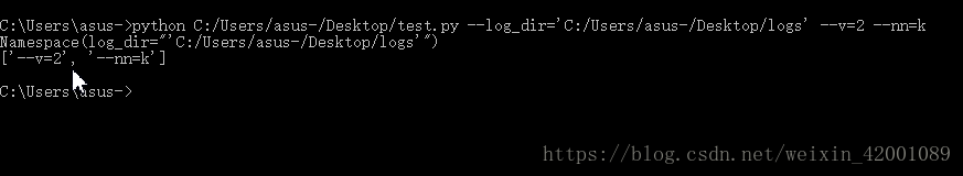
FLAGS, unparsed = parser.parse_known_args()print(FLAGS)
print(unparsed)
(三)接下来是下载数据集(这里稍微做了一点修改):
vocabulary_size = 50000def build_dataset(words, n_words):"""Process raw inputs into a dataset."""count = [['UNK', -1]]count.extend(collections.Counter(words).most_common(n_words - 1))dictionary = dict()for word, _ in count:dictionary[word] = len(dictionary)data = list()unk_count = 0for word in words:index = dictionary.get(word, 0)if index == 0:  # dictionary['UNK']unk_count += 1data.append(index)count[0][1] = unk_countreversed_dictionary = dict(zip(dictionary.values(), dictionary.keys()))return data, count, dictionary, reversed_dictionarydata, count, dictionary, reverse_dictionary = build_dataset(vocabulary, vocabulary_size)
del vocabulary  # Hint to reduce memory.
print('Most common words (+UNK)', count[:5])
print('Sample data', data[:10], [reverse_dictionary[i] for i in data[:10]])
其中下面是统计每个单词的词频,并选取前50000个词频较高的单词作为字典的备选词
extend追加一个列表
data_index = 0def generate_batch(batch_size, num_skips, skip_window):global data_indexassert batch_size % num_skips == 0assert num_skips <= 2 * skip_windowbatch = np.ndarray(shape=(batch_size), dtype=np.int32)labels = np.ndarray(shape=(batch_size, 1), dtype=np.int32)span = 2 * skip_window + 1  # [ skip_window target skip_window ]buffer = collections.deque(maxlen=span)  # pylint: disable=redefined-builtinif data_index + span > len(data):data_index = 0buffer.extend(data[data_index:data_index + span])data_index += spanfor i in range(batch_size // num_skips):context_words = [w for w in range(span) if w != skip_window]words_to_use = random.sample(context_words, num_skips)for j, context_word in enumerate(words_to_use):batch[i * num_skips + j] = buffer[skip_window]labels[i * num_skips + j, 0] = buffer[context_word]if data_index == len(data):buffer.extend(data[0:span])data_index = spanelse:buffer.append(data[data_index])data_index += 1# Backtrack a little bit to avoid skipping words in the end of a batchdata_index = (data_index + len(data) - span) % len(data)return batch, labelsbatch, labels = generate_batch(batch_size=8, num_skips=2, skip_window=1)
for i in range(8):print(batch[i], reverse_dictionary[batch[i]], '->', labels[i, 0],reverse_dictionary[labels[i, 0]])
batch_size:就是批次大小
num_skips:就是重复用一个单词的次数,比如 num_skips=2时,对于一句话:i love tensorflow very much ..........
当tensorflow被选为目标词时,在产生label时要利用tensorflow两次即:
tensorflow---》 love tensorflow---》 very
skip_window:是考虑左右上下文的个数,比如skip_window=1,就是在考虑上下文的时候,左面一个,右面一个
skip_window=2时,就是在考虑上下文的时候,左面两个,右面两个
span :其实在分批次的过程中可以看做是一个固定大小的框框(比较流行的说法数滑动窗口)在不断移动,而这个框框的大小 就是 span,可以看到span = 2 * skip_window + 1
buffer = collections.deque(maxlen=span):就是申请了一个buffer(其实就是固定大小的窗口这里是3)即每次这个buffer队列中最 多 能容纳span个单词
所以过程应该是这样的:比如batch_size=6, num_skips=2,skip_window=1,data:
batch_size // num_skips=3,循环3次
( I am looking for the missing glass-shoes who has picked it up .............)
2 23 56 3 45 84 123 45 23 12 1 14 ...............
i=0时:2 ,23 ,56首先进入 buffer( context_words = [w for w in range(span) if w != skip_window]的意思就是取窗口中不包括目标词 的词即上下文),然后batch[i * num_skips + j] = buffer[skip_window](skip_window=1,所以每次就是取窗口的中间数为 目标词)即batch=23, labels[i * num_skips + j, 0] = buffer[context_word]就是取其上下文为labels即2和56
所以此时batch=[23,23] labels=[2,56](当然也可能是[2,56],因为可能先取右边,后取左面),同时data_index=3即单词for的 位置
i=1时:data[data_index]进队列,即 buffer为 23,56,3 赋值后为:batch=[23,23,56,56] labels=[2,56,23,3](也可能是换一下顺序)
同时data_index=4即单词the
i=2时:data[data_index]进队列,即 buffer为 56,3,45 赋值后为:batch=[23,23,56,56,3,3] labels=[2,56,23,3,56,45](也可能是换一 下顺序) 同时data_index=5即单词missing
至此循环结束,按要求取出大小为6的一个批次即:
batch=[23,23,56,56,3,3] labels=[2,56,23,3,56,45]
然后data_index = (data_index + len(data) - span) % len(data)即data_index回溯3个单位,回到 looking,因为global data_index
所以data_index全局变量,所以当在取下一个批次的时候,buffer从looking的位置开始装载,即从上一个批次结束的位置接着往下取batch和labels
(七)定义一些参数大小:
with graph.as_default():# Input data.with tf.name_scope('inputs'):train_inputs = tf.placeholder(tf.int32, shape=[batch_size])train_labels = tf.placeholder(tf.int32, shape=[batch_size, 1])valid_dataset = tf.constant(valid_examples, dtype=tf.int32)# Ops and variables pinned to the CPU because of missing GPU implementationwith tf.device('/cpu:0'):# Look up embeddings for inputs.with tf.name_scope('embeddings'):embeddings = tf.Variable(tf.random_uniform([vocabulary_size, embedding_size], -1.0, 1.0))embed = tf.nn.embedding_lookup(embeddings, train_inputs)# Construct the variables for the NCE losswith tf.name_scope('weights'):nce_weights = tf.Variable(tf.truncated_normal([vocabulary_size, embedding_size],stddev=1.0 / math.sqrt(embedding_size)))with tf.name_scope('biases'):nce_biases = tf.Variable(tf.zeros([vocabulary_size]))# Compute the average NCE loss for the batch.# tf.nce_loss automatically draws a new sample of the negative labels each# time we evaluate the loss.# Explanation of the meaning of NCE loss:# http://mccormickml.com/2016/04/19/word2vec-tutorial-the-skip-gram-model/with tf.name_scope('loss'):loss = tf.reduce_mean(tf.nn.nce_loss(weights=nce_weights,biases=nce_biases,labels=train_labels,inputs=embed,num_sampled=num_sampled,num_classes=vocabulary_size))# Add the loss value as a scalar to summary.tf.summary.scalar('loss', loss)# Construct the SGD optimizer using a learning rate of 1.0.with tf.name_scope('optimizer'):optimizer = tf.train.GradientDescentOptimizer(1.0).minimize(loss)# Compute the cosine similarity between minibatch examples and all embeddings.norm = tf.sqrt(tf.reduce_sum(tf.square(embeddings), 1, keepdims=True))normalized_embeddings = embeddings / normvalid_embeddings = tf.nn.embedding_lookup(normalized_embeddings,valid_dataset)similarity = tf.matmul(valid_embeddings, normalized_embeddings, transpose_b=True)# Merge all summaries.merged = tf.summary.merge_all()# Add variable initializer.init = tf.global_variables_initializer()# Create a saver.saver = tf.train.Saver()这里可以分为两部分来看,一部分是训练Skip-gram模型的词向量,另一部分是计算余弦相似度,下面我们分开说:
首先看下tf.nn.embedding_lookup的API解释:
https://github.com/tensorflow/tensorflow/blob/master/tensorflow/python/ops/embedding_ops.py
def sigmoid_cross_entropy_with_logits( # pylint: disable=invalid-name_sentinel=None,labels=None,logits=None,name=None):"""Computes sigmoid cross entropy given `logits`.Measures the probability error in discrete classification tasks in which eachclass is independent and not mutually exclusive. For instance, one couldperform multilabel classification where a picture can contain both an elephantand a dog at the same time.For brevity, let `x = logits`, `z = labels`. The logistic loss isz * -log(sigmoid(x)) + (1 - z) * -log(1 - sigmoid(x))= z * -log(1 / (1 + exp(-x))) + (1 - z) * -log(exp(-x) / (1 + exp(-x)))= z * log(1 + exp(-x)) + (1 - z) * (-log(exp(-x)) + log(1 + exp(-x)))= z * log(1 + exp(-x)) + (1 - z) * (x + log(1 + exp(-x))= (1 - z) * x + log(1 + exp(-x))= x - x * z + log(1 + exp(-x))For x < 0, to avoid overflow in exp(-x), we reformulate the abovex - x * z + log(1 + exp(-x))= log(exp(x)) - x * z + log(1 + exp(-x))= - x * z + log(1 + exp(x))Hence, to ensure stability and avoid overflow, the implementation uses thisequivalent formulationmax(x, 0) - x * z + log(1 + exp(-abs(x)))`logits` and `labels` must have the same type and shape.Args:_sentinel: Used to prevent positional parameters. Internal, do not use.labels: A `Tensor` of the same type and shape as `logits`.logits: A `Tensor` of type `float32` or `float64`.name: A name for the operation (optional).Returns:A `Tensor` of the same shape as `logits` with the componentwiselogistic losses.Raises:ValueError: If `logits` and `labels` do not have the same shape."""# pylint: disable=protected-accessnn_ops._ensure_xent_args("sigmoid_cross_entropy_with_logits", _sentinel,labels, logits)# pylint: enable=protected-accesswith ops.name_scope(name, "logistic_loss", [logits, labels]) as name:logits = ops.convert_to_tensor(logits, name="logits")labels = ops.convert_to_tensor(labels, name="labels")try:labels.get_shape().merge_with(logits.get_shape())except ValueError:raise ValueError("logits and labels must have the same shape (%s vs %s)" %(logits.get_shape(), labels.get_shape()))# The logistic loss formula from above is# x - x * z + log(1 + exp(-x))# For x < 0, a more numerically stable formula is# -x * z + log(1 + exp(x))# Note that these two expressions can be combined into the following:# max(x, 0) - x * z + log(1 + exp(-abs(x)))# To allow computing gradients at zero, we define custom versions of max and# abs functions.zeros = array_ops.zeros_like(logits, dtype=logits.dtype)cond = (logits >= zeros)relu_logits = array_ops.where(cond, logits, zeros)neg_abs_logits = array_ops.where(cond, -logits, logits)return math_ops.add(relu_logits - logits * labels,math_ops.log1p(math_ops.exp(neg_abs_logits)),name=name)可以看到其实最关键的就是下面这个公式:
z * -log(sigmoid(x)) + (1 - z) * -log(1 - sigmoid(x))
其实z * -log(x) + (1 - z) * -log(1 - x)就是交叉熵,对的,没看错这个函数其实就是将输入先sigmoid再计算交叉熵
如上所示最后化简结果为:x - x * z + log(1 + exp(-x))
这里考虑到当x<0时exp(-x)有可能溢出,所以当x<0时有- x * z + log(1 + exp(x))
最后综合两种情况归纳出:
max(x, 0) - x * z + log(1 + exp(-abs(x)))
关于交叉熵的概念可以看一下:
https://blog.csdn.net/rtygbwwwerr/article/details/50778098
(3)最后看一下_sum_rows
num_steps = 100001with tf.Session(graph=graph) as session:# Open a writer to write summaries.writer = tf.summary.FileWriter(FLAGS.log_dir, session.graph)# We must initialize all variables before we use them.init.run()print('Initialized')average_loss = 0for step in xrange(num_steps):batch_inputs, batch_labels = generate_batch(batch_size, num_skips,skip_window)feed_dict = {train_inputs: batch_inputs, train_labels: batch_labels}# Define metadata variable.run_metadata = tf.RunMetadata()# We perform one update step by evaluating the optimizer op (including it# in the list of returned values for session.run()# Also, evaluate the merged op to get all summaries from the returned "summary" variable.# Feed metadata variable to session for visualizing the graph in TensorBoard._, summary, loss_val = session.run([optimizer, merged, loss],feed_dict=feed_dict,run_metadata=run_metadata)average_loss += loss_val# Add returned summaries to writer in each step.writer.add_summary(summary, step)# Add metadata to visualize the graph for the last run.if step == (num_steps - 1):writer.add_run_metadata(run_metadata, 'step%d' % step)if step % 2000 == 0:if step > 0:average_loss /= 2000# The average loss is an estimate of the loss over the last 2000 batches.print('Average loss at step ', step, ': ', average_loss)average_loss = 0# Note that this is expensive (~20% slowdown if computed every 500 steps)if step % 10000 == 0:sim = similarity.eval()for i in xrange(valid_size):valid_word = reverse_dictionary[valid_examples[i]]top_k = 8 # number of nearest neighborsnearest = (-sim[i, :]).argsort()[1:top_k + 1]log_str = 'Nearest to %s:' % valid_wordfor k in xrange(top_k):close_word = reverse_dictionary[nearest[k]]log_str = '%s %s,' % (log_str, close_word)print(log_str)final_embeddings = normalized_embeddings.eval()# Write corresponding labels for the embeddings.with open(FLAGS.log_dir + '/metadata.tsv', 'w') as f:for i in xrange(vocabulary_size):f.write(reverse_dictionary[i] + '\n')# Save the model for checkpoints.saver.save(session, os.path.join(FLAGS.log_dir, 'model.ckpt'))# Create a configuration for visualizing embeddings with the labels in TensorBoard.config = projector.ProjectorConfig()embedding_conf = config.embeddings.add()embedding_conf.tensor_name = embeddings.nameembedding_conf.metadata_path = os.path.join(FLAGS.log_dir, 'metadata.tsv')projector.visualize_embeddings(writer, config)writer.close()这部分源码简单易懂主要依次做了以下几件事:
(1)训练模型
(2)在训练最后一次,保存模型用以后续可视化
(3)每2000次,计算一次平均loss
(4)每10000次,打印(八)中随机选取16个词各自对应的与其最相近的8个词
(5)保存训练好的embeddings矩阵为.tsv格式用于在tensorboard通过降维来可视化
(6)保存模型为.ckpt
(十)二维可视化
def generate_batch(batch_size, cbow_window):global data_indexassert cbow_window % 2 == 1span = 2 * cbow_window + 1# 去除中心word: span - 1batch = np.ndarray(shape=(batch_size, span - 1), dtype=np.int32)labels = np.ndarray(shape=(batch_size, 1), dtype=np.int32)buffer = collections.deque(maxlen=span)for _ in range(span):buffer.append(data[data_index])# 循环选取 data中数据,到尾部则从头开始data_index = (data_index + 1) % len(data)for i in range(batch_size):# target at the center of spantarget = cbow_window# 仅仅需要知道context(word)而不需要wordtarget_to_avoid = [cbow_window]col_idx = 0for j in range(span):# 略过中心元素 wordif j == span // 2:continuebatch[i, col_idx] = buffer[j]col_idx += 1labels[i, 0] = buffer[target]# 更新 bufferbuffer.append(data[data_index])data_index = (data_index + 1) % len(data)return batch, labelsbatch, labels = generate_batch(batch_size=8, cbow_window=1)
for i in range(8):print(reverse_dictionary[batch[i,0]],'and',reverse_dictionary[batch[i,1]] ,'->', reverse_dictionary[labels[i, 0]])
with graph.as_default():# Input data.with tf.name_scope('inputs'):train_dataset = tf.placeholder(tf.int32, shape=[batch_size,2 * cbow_window])train_labels = tf.placeholder(tf.int32, shape=[batch_size, 1])valid_dataset = tf.constant(valid_examples, dtype=tf.int32)# Ops and variables pinned to the CPU because of missing GPU implementationwith tf.device('/cpu:0'):# Look up embeddings for inputs.with tf.name_scope('embeddings'):embeddings = tf.Variable(tf.random_uniform([vocabulary_size, embedding_size], -1.0, 1.0))# Construct the variables for the NCE losswith tf.name_scope('weights'):nce_weights = tf.Variable(tf.truncated_normal([vocabulary_size, embedding_size],stddev=1.0 / math.sqrt(embedding_size)))with tf.name_scope('biases'):nce_biases = tf.Variable(tf.zeros([vocabulary_size]))embeds = Nonefor i in range(2 * cbow_window):embedding_i = tf.nn.embedding_lookup(embeddings, train_dataset[:,i])print('embedding %d shape: %s'%(i, embedding_i.get_shape().as_list()))emb_x,emb_y = embedding_i.get_shape().as_list()if embeds is None:embeds = tf.reshape(embedding_i, [emb_x,emb_y,1])else:embeds = tf.concat([embeds, tf.reshape(embedding_i, [emb_x, emb_y,1])], 2)print("Concat embedding size: %s"%embeds.get_shape().as_list())avg_embed = tf.reduce_mean(embeds, 2, keep_dims=False)print("Avg embedding size: %s"%avg_embed.get_shape().as_list())print('--------------------------------------------------------------------------------------------')print(avg_embed.shape)print(train_labels.shape)print('--------------------------------------------------------------------------------------------')# Compute the average NCE loss for the batch.# tf.nce_loss automatically draws a new sample of the negative labels each# time we evaluate the loss.# Explanation of the meaning of NCE loss:# http://mccormickml.com/2016/04/19/word2vec-tutorial-the-skip-gram-model/with tf.name_scope('loss'):loss = tf.reduce_mean(tf.nn.nce_loss(weights=nce_weights,biases=nce_biases,labels=train_labels,inputs=avg_embed,num_sampled=num_sampled,num_classes=vocabulary_size))# Add the loss value as a scalar to summary.tf.summary.scalar('loss', loss)# Construct the SGD optimizer using a learning rate of 1.0.with tf.name_scope('optimizer'):optimizer = tf.train.GradientDescentOptimizer(1.0).minimize(loss)# Compute the cosine similarity between minibatch examples and all embeddings.norm = tf.sqrt(tf.reduce_sum(tf.square(embeddings), 1, keepdims=True))normalized_embeddings = embeddings / normvalid_embeddings = tf.nn.embedding_lookup(normalized_embeddings,valid_dataset)similarity = tf.matmul(valid_embeddings, normalized_embeddings, transpose_b=True)# Merge all summaries.merged = tf.summary.merge_all()# Add variable initializer.init = tf.global_variables_initializer()# Create a saver.saver = tf.train.Saver()
这里的特殊之处在于怎么将batch和labels维数对应
以下假设embeding的特征数都是128
对于Skip-Gram模型模型
经过generate_batch后返回:
batch:batch_size
labels : batch_size*1
然后 经过(八)的(train_inputs=batch) embed = tf.nn.embedding_lookup(embeddings, train_inputs)后
embed : batch_size*128
labels : batch_size*1
所以传给 tf.nn.nce_loss进行训练的
此时对于CBOW模型
经过generate_batch后返回:
batch:batch_size*span - 1(batch_size*2)
labels : batch_size*1
如果还是按照Skip-Gram模型则
经过(八)的(train_inputs=batch) embed = tf.nn.embedding_lookup(embeddings, train_inputs)后
会报错,而且原先Skip-Gram中目标词汇是一个,现在CBOW中目标词汇是两个
基于此本程序是进行如下处理来产生embed 的:
首先先遍历目标词汇的一个(i=0),通过 embedding_i = tf.nn.embedding_lookup(embeddings, train_dataset[:,i])
此时embedding_i维度为batch_size*128然后reshape为batch_size*128*1
然后将embedding_i赋给 embeds
接着再遍历目标词中剩下的一个(i=1),通过 embedding_i = tf.nn.embedding_lookup(embeddings, train_dataset[:,i])
此时embedding_i维度为batch_size*128然后reshape为batch_size*128*1
然后再将embedding_i合并到embeds(合并的维度是2)此时embeds维度为batch_size*128*2
然后avg_embed = tf.reduce_mean(embeds, 2, keep_dims=False)后avg_embed维数为batch_size*128
最后将
avg_embed : batch_size*128
labels: batch_size*1
所以传给 tf.nn.nce_loss进行训练的
这样说不是很直观下面举个类子(batch_size=8)
即比如batch为[ [ 1 , 2 ] , [ 3 , 4 ], [ 5 , 6 ], [ 7 , 8 ], [ 9 , 10 ], [ 11 , 12 ], [ 13 , 14 ], [ 15 , 16 ]]
embeddings为 [ [ 1.1 , 1.2 ,1.3 ,.....................................................1.128]
[ 2.1 , 2.2 ,2.3 ,.....................................................2.128]
[ 3.1 , 3.2 ,3.3 ,.....................................................3.128]
................................
[ 50000.1 , 50000.2 ,50000.3 ,..................50000.128]
]
那么embeds为 [ [ [1.1 , 2.1] , [1.2 , 2.2] , [1.3 , 2.3] .......... , [1.128 , 2.128] ]
[ [3.1 , 4.1] , [3.2 , 4.2] , [3.3 , 4.3] .......... , [3.128 , 4.128] ]
[ [5.1 , 6.1] , [5.2 ,6.2] , [5.3 , 6.3] .......... , [5.128 , 6.128] ]
[ [7.1 , 8.1] , [7.2 , 8.2] , [7.3 , 8.3] .......... , [7.128 , 8.128] ]
[ [9.1 , 10.1] , [9.2 , 10.2] , [9.3 , 10.3] .......... , [9.128 , 10.128] ]
[ [11.1 , 12.1] , [11.2 , 12.2] , [11.3 , 12.3] .......... , [11.128 , 12.128] ]
[ [13.1 , 14.1] , [13.2 , 14.2] , [13.3 , 14.3] .......... , [13.128 , 14.128] ]
[ [15.1 , 16.1] , [15.2 , 16.2] , [15.3 , 16.3] .......... , [15.128 , 16.128] ]
]
avg_embed为
[ [ [ 3.2 ] , [ 3.4 ] , [ 3.6 ] .......... , [ 3.256 ] ]
[ [ 7.2 ] , [ 7.4 ] , [ 7.6 ] .......... , [ 7.256 ] ]
[ [ 11.2 ] , [ 11.4 ] , [11.6 ] .......... , [ 11.256 ] ]
.........................
[ [ 31.2 ] , [ 31.4 ] , [ 31.6 ] .......... , [ 31.256 ] ]
]
可以看出CBOW模型其实就是将目标词汇中的两个词对应的128个特征分别相加,整体作为一个输入的
其他代码就与Skip-Gram模型基本相同了
-----------------------------------------------------------------------------------------------------------------------------------------------------------------------------------
以下为运行结果的部分截图:

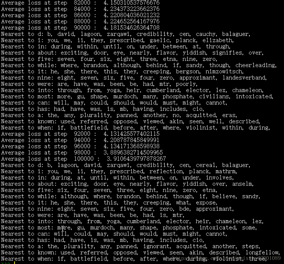
可以看到最后一步的loss为3.91,而Skip-Gram最后一步的loss为4.69,所以CBOW模型训练的结果更好一点,是因为其同时考虑了两个词去预测一个词,而Skip-Gram是用一个词去预测上下文
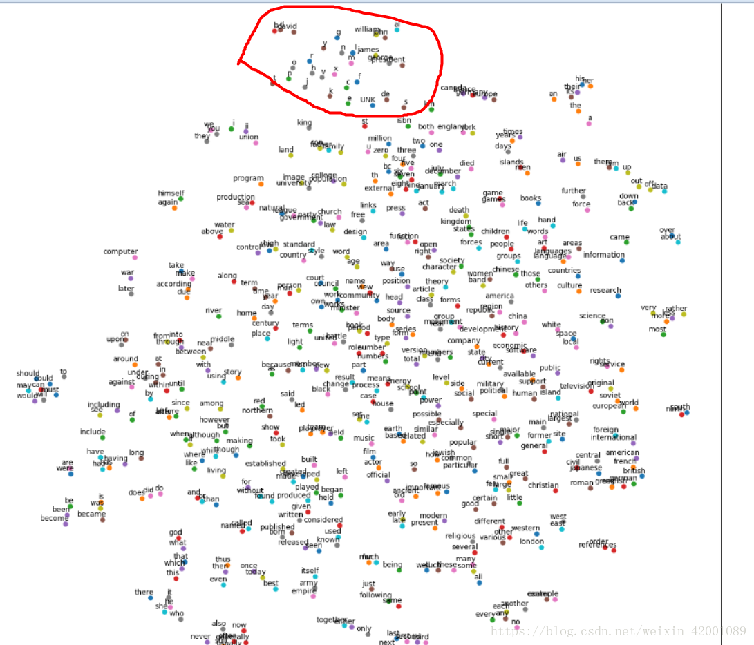
可视化也可以看到结果
tensorboard中的可视化:

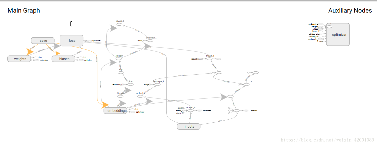

记得点红色的部分就能看到三维的分布了
###################################################################################################
全部代码:https://github.com/Mryangkaitong/tensorflow/tree/master/word2vec
关于可视化,可以使用tensorboard内置的embedding工具进行可视化,可以参考:
https://blog.csdn.net/szj_huhu/article/details/75308970
http://www.360doc.com/content/17/0706/14/10408243_669327270.shtml
等等
或者将数据集制作成.csv,直接在tensorboard内置的embedding的工具中加载:
地址为:http://projector.tensorflow.org/
https://blog.csdn.net/u010099080/article/details/53560426?fps=1&locationNum=11
关于怎样制作.csv可以参考:
https://jingyan.baidu.com/article/9c69d48ff3123d13c9024e06.html
本文来自互联网用户投稿,文章观点仅代表作者本人,不代表本站立场,不承担相关法律责任。如若转载,请注明出处。 如若内容造成侵权/违法违规/事实不符,请点击【内容举报】进行投诉反馈!