深度学习和目标检测系列教程 12-300：常见的opencv的APi和用法总结

@Author：Runsen

由于CV需要熟练使用opencv，因此总结了opencv常见的APi和用法。

OpenCV（opensourcecomputervision）于1999年正式推出，它来自英特尔的一项倡议。

• OpenCV的核心是用C++编写的。在Python中，我们只使用一个包装器，它在Python内部执行C++代码。

• 它对于几乎所有的计算机视觉应用程序都非常有用，并且在Windows、Linux、MacOS、Android、iOS上受支持，并绑定到Python、Java和Matlab。

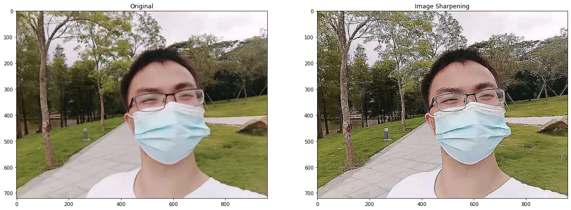
锐化

USM锐化的全称是：Unsharp Mask，译为「模糊掩盖锐化处理」，是一种胶片时代处理图片锐度的手法，延续到数码时代的产物。在胶片时代，我们通过将模糊的负片与正片叠加可产生边缘锐化的效果。

对，锐化的效果离不开模糊，甚至可以说，锐化的效果就是来源于模糊。USM的锐化实际上就是利用原图和模糊图产生的反差，来实现锐化图片的效果。

公式：（源图像– w*高斯模糊）/（1-w）；其中w表示权重（0.1～0.9）。

我感觉我喜欢上，毕业前在学校自拍的照片

import numpy as np
import matplotlib.pyplot as plt
import cv2image = cv2.imread('demo.jpg')
image = cv2.cvtColor(image, cv2.COLOR_BGR2RGB)plt.figure(figsize=(20, 20))
plt.subplot(1, 2, 1)
plt.title("Original")
plt.imshow(image)# Create our shapening kernel
# the values in the matrix sum to 1
kernel_sharpening = np.array([[-1,-1,-1], [-1,9,-1], [-1,-1,-1]])# 对输入图像应用不同的内核
sharpened = cv2.filter2D(image, -1, kernel_sharpening)plt.subplot(1, 2, 2)
plt.title("Image Sharpening")
plt.imshow(sharpened)plt.show()

阈值化、二值化

image = cv2.imread('demo.jpg', 0)plt.figure(figsize=(30, 30))
plt.subplot(3, 2, 1)
plt.title("Original")
plt.imshow(image)# 小于127的值变为0（黑色，大于等于255（白色）
ret,thresh1 = cv2.threshold(image, 127, 255, cv2.THRESH_BINARY)plt.subplot(3, 2, 2)
plt.title("Threshold Binary")
plt.imshow(thresh1)# 模糊图像，消除噪音
image = cv2.GaussianBlur(image, (3, 3), 0)#  adaptiveThreshold
thresh = cv2.adaptiveThreshold(image, 255, cv2.ADAPTIVE_THRESH_MEAN_C, cv2.THRESH_BINARY, 3, 5) plt.subplot(3, 2, 3)
plt.title("Adaptive Mean Thresholding")
plt.imshow(thresh)_, th2 = cv2.threshold(image, 0, 255, cv2.THRESH_BINARY + cv2.THRESH_OTSU)plt.subplot(3, 2, 4)
plt.title("Otsu's Thresholding")
plt.imshow(th2)plt.subplot(3, 2, 5)
# 高斯滤波后的大津阈值法
blur = cv2.GaussianBlur(image, (5,5), 0)
_, th3 = cv2.threshold(blur, 0, 255, cv2.THRESH_BINARY + cv2.THRESH_OTSU)
plt.title("Guassian Otsu's Thresholding")
plt.imshow(th3)
plt.show()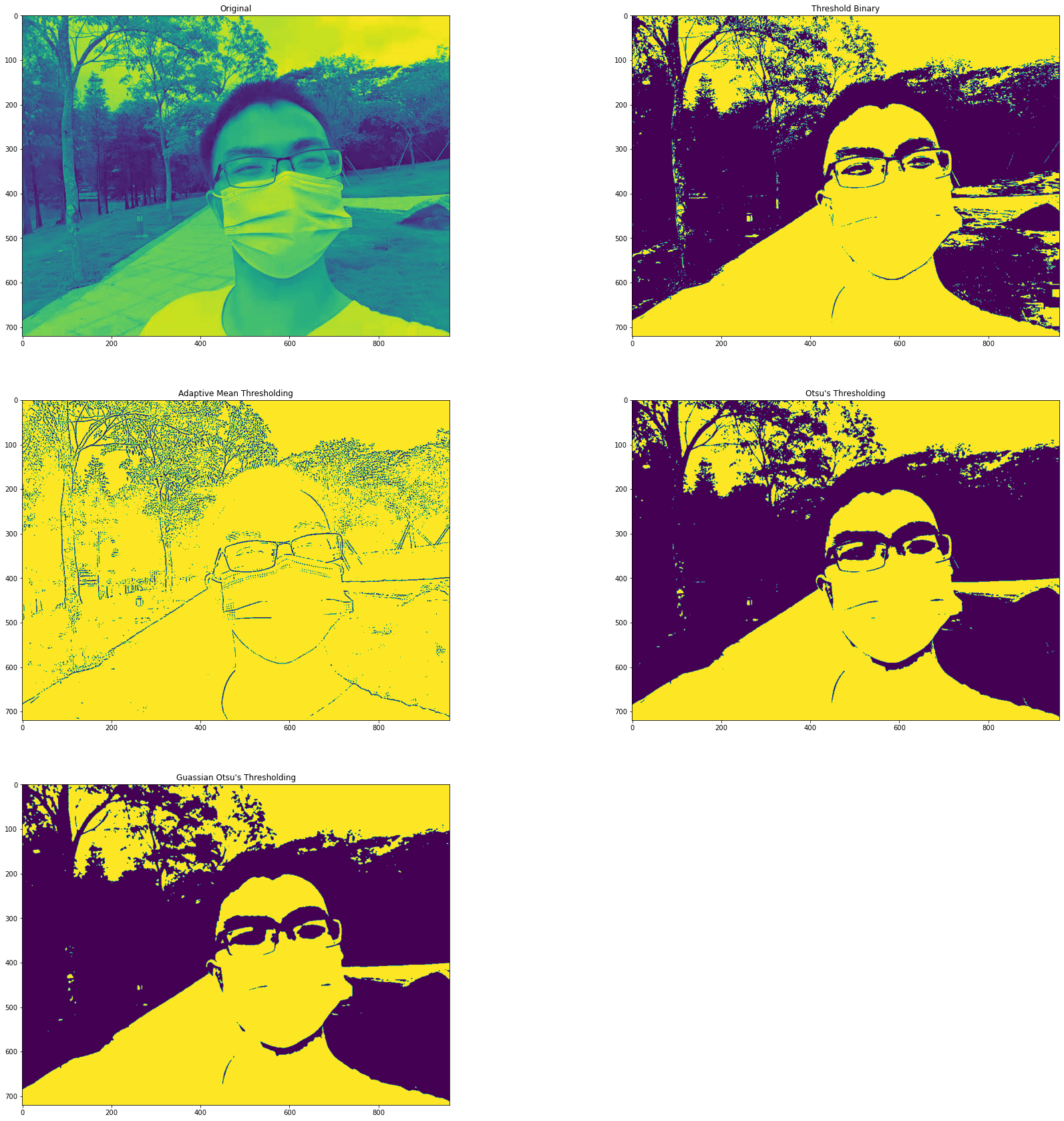

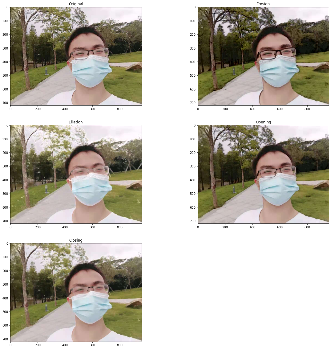
降噪

image = cv2.imread('demo.jpg')
image = cv2.cvtColor(image, cv2.COLOR_BGR2RGB)plt.figure(figsize=(20, 20))
plt.subplot(3, 2, 1)
plt.title("Original")
plt.imshow(image)# Let's define our kernel size
kernel = np.ones((5,5), np.uint8)# Now we erode
erosion = cv2.erode(image, kernel, iterations = 1)plt.subplot(3, 2, 2)
plt.title("Erosion")
plt.imshow(erosion)dilation = cv2.dilate(image, kernel, iterations = 1)
plt.subplot(3, 2, 3)
plt.title("Dilation")
plt.imshow(dilation)# Opening - Good for removing noise
opening = cv2.morphologyEx(image, cv2.MORPH_OPEN, kernel)
plt.subplot(3, 2, 4)
plt.title("Opening")
plt.imshow(opening)# Closing - Good for removing noise
closing = cv2.morphologyEx(image, cv2.MORPH_CLOSE, kernel)
plt.subplot(3, 2, 5)
plt.title("Closing")
plt.imshow(closing)

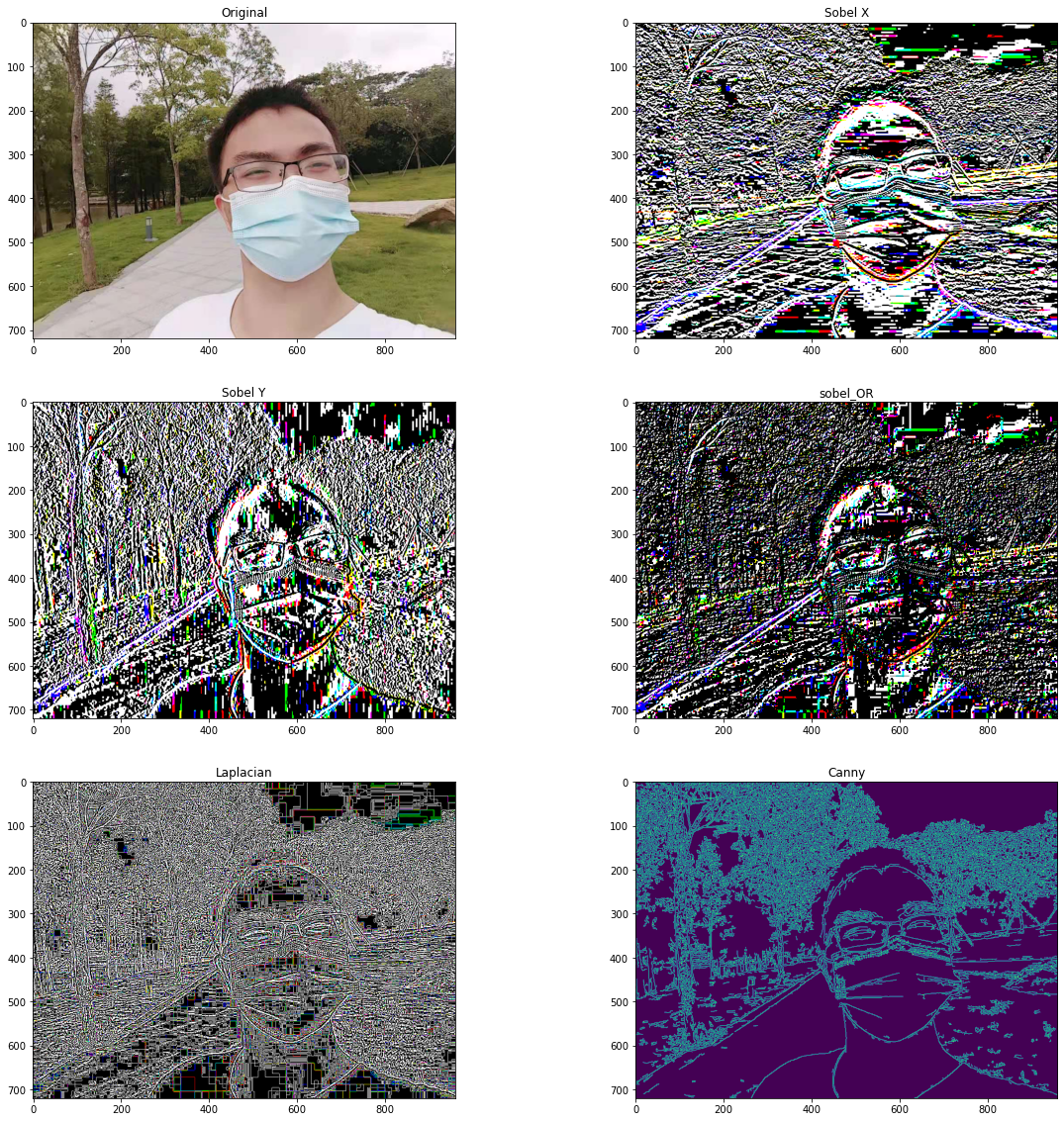
边缘检测与图像梯度

image = cv2.imread('demo.jpg')
image = cv2.cvtColor(image, cv2.COLOR_BGR2RGB)height, width,_ = image.shape# Extract Sobel Edges
sobel_x = cv2.Sobel(image, cv2.CV_64F, 0, 1, ksize=5)
sobel_y = cv2.Sobel(image, cv2.CV_64F, 1, 0, ksize=5)plt.figure(figsize=(20, 20))plt.subplot(3, 2, 1)
plt.title("Original")
plt.imshow(image)plt.subplot(3, 2, 2)
plt.title("Sobel X")
plt.imshow(sobel_x)plt.subplot(3, 2, 3)
plt.title("Sobel Y")
plt.imshow(sobel_y)sobel_OR = cv2.bitwise_or(sobel_x, sobel_y)plt.subplot(3, 2, 4)
plt.title("sobel_OR")
plt.imshow(sobel_OR)laplacian = cv2.Laplacian(image, cv2.CV_64F)plt.subplot(3, 2, 5)
plt.title("Laplacian")
plt.imshow(laplacian)## 提供两个值：threshold1和threshold2。任何大于threshold2的梯度值。低于threshold1的任何值都不被视为边。
# threshold1和threshold2之间的值可以根据其大小分类为边或非边 
# 在这种情况下，低于60的任何渐变值都被视为非边
# 而大于120的任何值都被视为边。
# The first threshold gradient
canny = cv2.Canny(image, 50, 120)plt.subplot(3, 2, 6)
plt.title("Canny")
plt.imshow(canny)

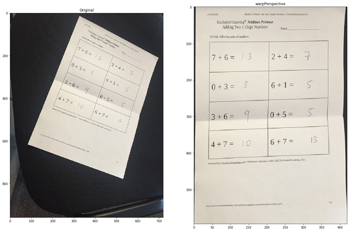
透视变换

image = cv2.imread('scan.jpg')
image = cv2.cvtColor(image, cv2.COLOR_BGR2RGB)plt.figure(figsize=(20, 20))plt.subplot(1, 2, 1)
plt.title("Original")
plt.imshow(image)# 原始图像四个角的坐标
points_A = np.float32([[320,15], [700,215], [85,610], [530,780]])# 所需输出的4个角的坐标
# 使用A4纸的比例是1:1.41
points_B = np.float32([[0,0], [420,0], [0,594], [420,594]])# 使用两组四个点进行计算
# 透视变换矩阵，M 
M = cv2.getPerspectiveTransform(points_A, points_B)warped = cv2.warpPerspective(image, M, (420,594))plt.subplot(1, 2, 2)
plt.title("warpPerspective")
plt.imshow(warped)

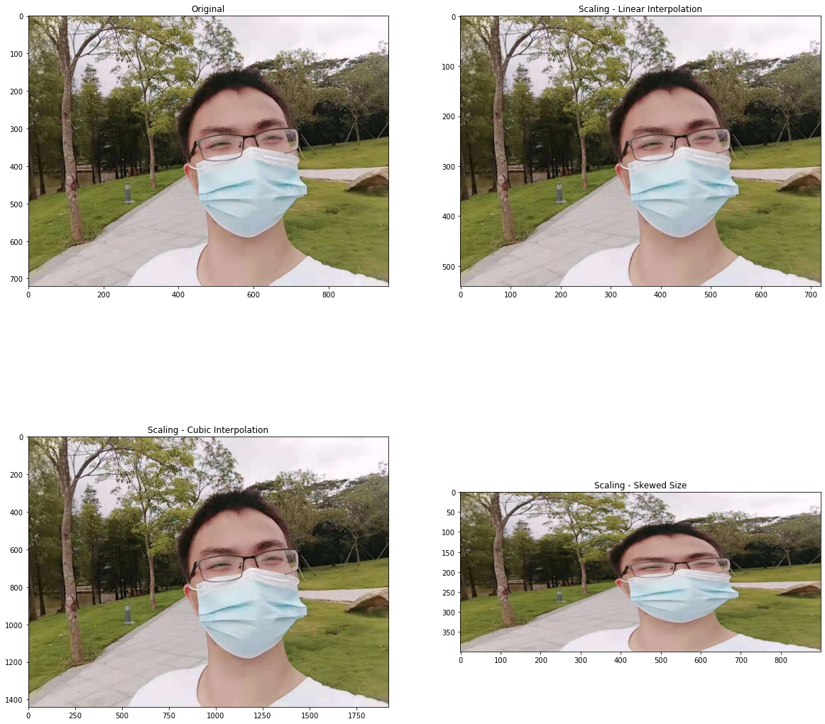
缩放、重新调整大小和插值

使用cv2.resize函数可以很容易地重新调整大小，它的参数有：cv2.resize（image，dsize（output image size），x scale，y scale，interpolation）

image = cv2.imread('demo.jpg')
image = cv2.cvtColor(image, cv2.COLOR_BGR2RGB)plt.figure(figsize=(20, 20))plt.subplot(2, 2, 1)
plt.title("Original")
plt.imshow(image)# Let's make our image 3/4 of it's original size
image_scaled = cv2.resize(image, None, fx=0.75, fy=0.75)plt.subplot(2, 2, 2)
plt.title("Scaling - Linear Interpolation")
plt.imshow(image_scaled)# Let's double the size of our image
img_scaled = cv2.resize(image, None, fx=2, fy=2, interpolation = cv2.INTER_CUBIC)plt.subplot(2, 2, 3)
plt.title("Scaling - Cubic Interpolation")
plt.imshow(img_scaled)# Let's skew the re-sizing by setting exact dimensions
img_scaled = cv2.resize(image, (900, 400), interpolation = cv2.INTER_AREA)plt.subplot(2, 2, 4)
plt.title("Scaling - Skewed Size")
plt.imshow(img_scaled)

影像金字塔

在目标检测中缩放图像时非常有用。

image = cv2.imread('demo.jpg')
image = cv2.cvtColor(image, cv2.COLOR_BGR2RGB)plt.figure(figsize=(20, 20))plt.subplot(2, 2, 1)
plt.title("Original")
plt.imshow(image)smaller = cv2.pyrDown(image)
larger = cv2.pyrUp(image)plt.subplot(2, 2, 2)
plt.title("Smaller")
plt.imshow(smaller)plt.subplot(2, 2, 3)
plt.title("Larger")
plt.imshow(larger)

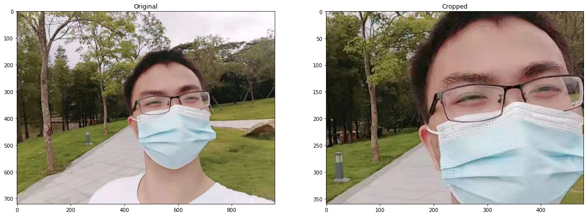
裁剪

image = cv2.imread('demo.jpg')
image = cv2.cvtColor(image, cv2.COLOR_BGR2RGB)plt.figure(figsize=(20, 20))plt.subplot(2, 2, 1)
plt.title("Original")
plt.imshow(image)height, width = image.shape[:2]# Let's get the starting pixel coordiantes (top  left of cropping rectangle)
start_row, start_col = int(height * .25), int(width * .25)# Let's get the ending pixel coordinates (bottom right)
end_row, end_col = int(height * .75), int(width * .75)# Simply use indexing to crop out the rectangle we desire
cropped = image[start_row:end_row , start_col:end_col]plt.subplot(2, 2, 2)
plt.title("Cropped")
plt.imshow(cropped)

模糊

image = cv2.imread('demo.jpg')
image = cv2.cvtColor(image, cv2.COLOR_BGR2RGB)plt.figure(figsize=(20, 20))plt.subplot(2, 2, 1)
plt.title("Original")
plt.imshow(image)# Creating our 3 x 3 kernel
kernel_3x3 = np.ones((3, 3), np.float32) / 9# We use the cv2.fitler2D to conovlve the kernal with an image 
blurred = cv2.filter2D(image, -1, kernel_3x3)plt.subplot(2, 2, 2)
plt.title("3x3 Kernel Blurring")
plt.imshow(blurred)# Creating our 7 x 7 kernel
kernel_7x7 = np.ones((7, 7), np.float32) / 49blurred2 = cv2.filter2D(image, -1, kernel_7x7)plt.subplot(2, 2, 3)
plt.title("7x7 Kernel Blurring")
plt.imshow(blurred2)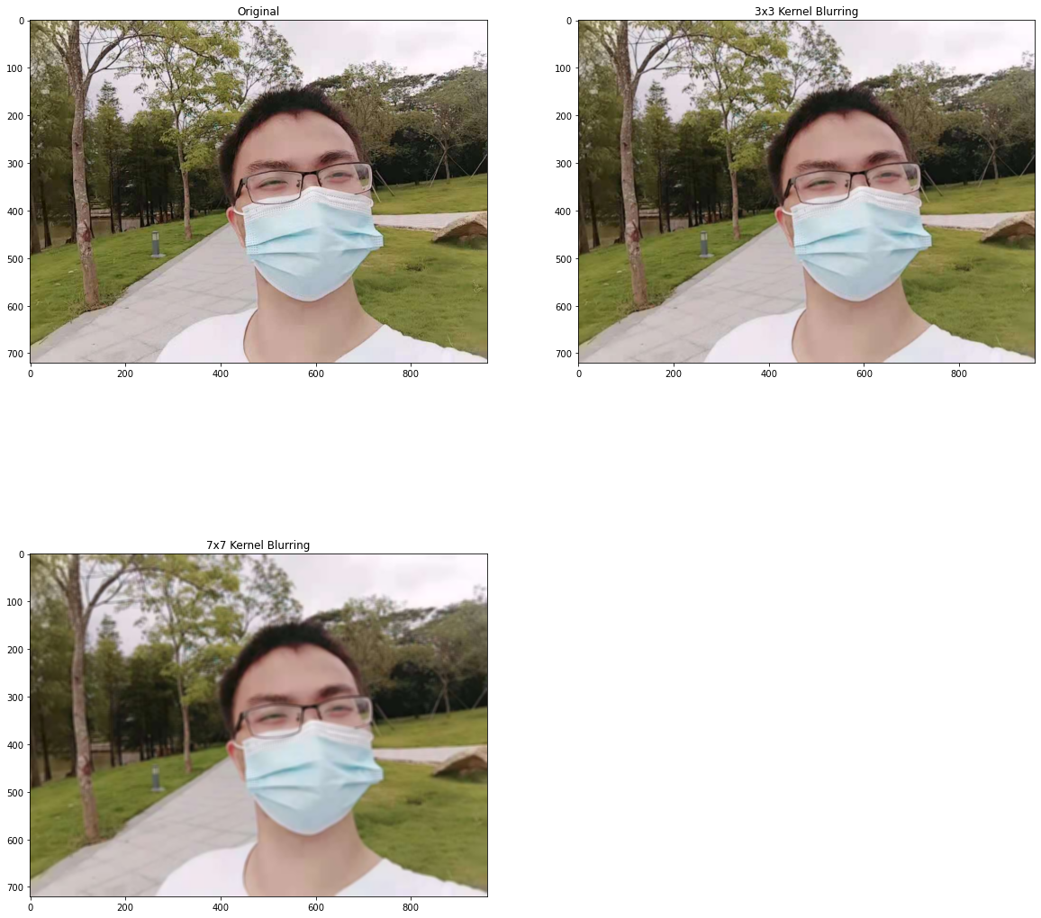

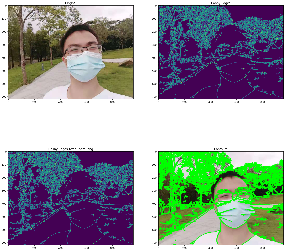
Contours

# Let's load a simple image with 3 black squares
image = cv2.imread('demo.jpg')
image = cv2.cvtColor(image, cv2.COLOR_BGR2RGB)plt.figure(figsize=(20, 20))plt.subplot(2, 2, 1)
plt.title("Original")
plt.imshow(image)# Grayscale
gray = cv2.cvtColor(image,cv2.COLOR_BGR2GRAY)# Find Canny edges
edged = cv2.Canny(gray, 30, 200)plt.subplot(2, 2, 2)
plt.title("Canny Edges")
plt.imshow(edged)# Finding Contours
# Use a copy of your image e.g. edged.copy(), since findContours alters the image
contours, hierarchy = cv2.findContours(edged, cv2.RETR_EXTERNAL, cv2.CHAIN_APPROX_NONE)plt.subplot(2, 2, 3)
plt.title("Canny Edges After Contouring")
plt.imshow(edged)print("Number of Contours found = " + str(len(contours)))# Draw all contours
# Use '-1' as the 3rd parameter to draw all
cv2.drawContours(image, contours, -1, (0,255,0), 3)plt.subplot(2, 2, 4)
plt.title("Contours")
plt.imshow(image)

本文来自互联网用户投稿，文章观点仅代表作者本人，不代表本站立场，不承担相关法律责任。如若转载，请注明出处。 如若内容造成侵权/违法违规/事实不符，请点击【内容举报】进行投诉反馈！