TensorFlow学习（一）——常用方法

笔者是一个痴迷于挖掘数据中的价值的学习人，希望在平日的工作学习中，挖掘数据的价值，找寻数据的秘密，笔者认为，数据的价值不仅仅只体现在企业中，个人也可以体会到数据的魅力，用技术力量探索行为密码，让大数据助跑每一个人，欢迎直筒们关注我的公众号，大家一起讨论数据中的那些有趣的事情。

我的公众号为：livandata

一、tensorflow的常用函数：

import tensorflow as tf

import numpy as np

1.1、数据的呈现（Variable（）：定义变量）：

    x=np.array([[1,1,1],[1,-8,1],[1,1,1]])

    w=tf.Variable(initial_value=x)

    w=tf.Variable(tf.zeros([3,3]))

    init=tf.global_variables_initializer()

    withtf.Session() as sess:

           sess.run(init)

           print(sess.run(w))

1.2、数据的加减运算（add():加；multiply():乘）：

    a=tf.placeholder(tf.int16)

    b=tf.placeholder(tf.int16)

    add=tf.add(a,b)

    mul=tf.multiply(a,b)

    withtf.Session() as sess:

           print("a+b=", sess.run(add,feed_dict={a:2, b:3}))

           print("a*b=", sess.run(mul,feed_dict={a:2, b:3}))

1.3、矩阵相乘（matmul）运算：

    a=tf.Variable(tf.ones([3,3]))

    b=tf.Variable(tf.ones([3,3]))

    product=tf.matmul(tf.multiply(5.0,a),tf.multiply(4.0,b))

    init=tf.initialize_all_variables()

    withtf.Session() as sess:

           sess.run(init)

           print(sess.run(product))

1.4、argmax的练习：获取最大值的下标向量

a=tf.get_variable(name='a',shape=[3,4],dtype=tf.float32,initializer=tf.random_uniform_initializer(minval=-1,maxval=1))

    # 最大值所在的下标向量

    b=tf.argmax(input=a,axis=0)

    c=tf.argmax(input=a,dimension=1)

    sess=tf.InteractiveSession()

    sess.run(tf.initialize_all_variables())

    print(sess.run(a))

    print(sess.run(b))

    print(sess.run(c))

1.5、创建全一/全零矩阵：

  tf.ones(shape,type=tf.float32,name=None)

  tf.ones([2, 3], int32) ==> [[1, 1, 1], [1, 1, 1]]

  tf.zeros(shape,type=tf.float32,name=None)

  tf.zeros([2, 3], int32) ==> [[0, 0, 0],[0, 0, 0]]

1.7、tf.ones_like(tensor,dype=None,name=None)

  新建一个与给定的tensor类型大小一致的tensor，其所有元素为1。

    # 'tensor' is [[1, 2, 3], [4, 5, 6]] 

    tf.ones_like(tensor) ==> [[1, 1, 1], [1, 1, 1]]

1.8、tf.zeros_like(tensor,dype=None,name=None)

    新建一个与给定的tensor类型大小一致的tensor，其所有元素为0。

    # 'tensor' is [[1, 2, 3], [4, 5, 6]] 

    tf.ones_like(tensor) ==> [[0, 0, 0],[0, 0, 0]]

1.9、tf.fill(dim,value,name=None)

     创建一个形状大小为dim的tensor，其初始值为value

    # Output tensor has shape [2, 3]. 

    fill([2, 3], 9) ==> [[9, 9, 9] 

                               [9, 9, 9]]

1.10、tf.constant(value,dtype=None,shape=None,name='Const')

    创建一个常量tensor，先给出value，可以设定其shape

    # Constant 1-D Tensor populated with value list. 

    tensor = tf.constant([1, 2, 3, 4, 5, 6, 7]) => [1 2 3 4 5 67] 

     # Constant 2-D tensor populated with scalarvalue -1. 

    tensor = tf.constant(-1.0, shape=[2, 3]) => [[-1. -1. -1.] [-1.-1. -1.]

1.11、tf.linspace(start,stop,num,name=None)

     返回一个tensor，该tensor中的数值在start到stop区间之间取等差数列（包含start和stop），如果num>1则差值为(stop-start)/(num-1)，以保证最后一个元素的值为stop。

     其中，start和stop必须为tf.float32或tf.float64。num的类型为int。

    tf.linspace(10.0, 12.0, 3, name="linspace") => [ 10.011.0 12.0]

1.12、tf.range(start,limit=None,delta=1,name='range')

     返回一个tensor等差数列，该tensor中的数值在start到limit之间，不包括limit，delta是等差数列的差值。

     start，limit和delta都是int32类型。

    # 'start' is 3 

    # 'limit' is 18 

    # 'delta' is 3

    tf.range(start, limit, delta) ==> [3, 6, 9, 12, 15] 

    # 'limit' is 5 start is 0

    tf.range(start, limit) ==> [0, 1, 2, 3, 4]

1.13、tf.random_normal(shape,mean=0.0,stddev=1.0,dtype=tf.float32,seed=None,name=None)

    返回一个tensor其中的元素的值服从正态分布。

    seed: A Python integer. Used to create a random seed for thedistribution.See set_random_seed forbehavior。

1.14、tf.truncated_normal(shape, mean=0.0, stddev=1.0, dtype=tf.float32,seed=None, name=None)

     返回一个tensor其中的元素服从截断正态分布（？概念不懂，留疑）

1.15、tf.random_uniform(shape,minval=0,maxval=None,dtype=tf.float32,seed=None,name=None)

     返回一个形状为shape的tensor，其中的元素服从minval和maxval之间的均匀分布。

1.16、tf.random_shuffle(value,seed=None,name=None)

    对value（是一个tensor）的第一维进行随机化。

      [[1,2],               [[2,3],

       [2,3],        ==>  [1,2],

       [3,4]]                [3,4]] 

1.17、tf.set_random_seed(seed)

    设置产生随机数的种子。

二、常规神经网络（NN）：

import tensorflow as tf

import tensorflow.examples.tutorials.mnist.input_data as input_data

mnist=input_data.read_data_sets("Mnist_data/", one_hot=True)

# val_data=mnist.validation.images

# val_label=mnist.validation.labels

#print("______________________________")

# print(mnist.train.images.shape)

# print(mnist.train.labels.shape)

# print(mnist.validation.images.shape)

# print(mnist.validation.labels.shape)

# print(mnist.test.images.shape)

# print(mnist.test.labels.shape)

# print(val_data)

# print(val_label)

# print("==============================") 

x = tf.placeholder(tf.float32, [None,784])

y_actual = tf.placeholder(tf.float32, shape=[None,10])

W = tf.Variable(tf.zeros([784,10]))

b = tf.Variable(tf.zeros([10]))

y_predict = tf.nn.softmax(tf.matmul(x, W)+b)

cross_entropy=tf.reduce_mean(-tf.reduce_sum(y_actual*tf.log(y_predict),reduction_indices=1))

train_step=tf.train.GradientDescentOptimizer(0.01).minimize(cross_entropy)

correct_prediction=tf.equal(tf.argmax(y_predict,1),tf.argmax(y_actual, 1))

accuracy=tf.reduce_mean(tf.cast(correct_prediction,"float"))

init = tf.initialize_all_variables()

with tf.Session() assess:

   sess.run(init)

    fori in range(1000):

       batch_xs, batch_ys = mnist.train.next_batch(100)

       sess.run(train_step, feed_dict={x:batch_xs, y_actual:batch_ys})

       if(i%100==0):

           print("accuracy:" ,sess.run(accuracy, feed_dict={x:mnist.test.images,y_actual:mnist.test.labels}))

三、线性网络模型：

import tensorflow as tf

import numpy as np

# 用numpy随机生成100个数：

x_data=np.float32(np.random.rand(2,100))

y_data=np.dot([0.100,0.200], x_data)+0.300

# 构造一个线性模型：

b=tf.Variable(tf.zeros([1]))

W=tf.Variable(tf.random_uniform([1,2],-1.0, 1.0))

y=tf.matmul(W, x_data)+b

# 最小化方差

loss=tf.reduce_mean(tf.square(y-y_data))

optimizer=tf.train.GradientDescentOptimizer(0.5)

train = optimizer.minimize(loss)

# 初始化变量

init=tf.initialize_all_variables()

# 启动图

sess=tf.Session()

sess.run(init)

# 拟合平面

for step inrange(0, 201):

   sess.run(train)

    ifstep % 20 == 0:

       print(step,sess.run(W), sess.run(b))

四、CNN卷积神经网络：

# -*- coding: utf-8 -*-

"""

Created on ThuSep  8 15:29:48 2016

@author: root

"""

import tensorflow as tf

import tensorflow.examples.tutorials.mnist.input_data asinput_data

mnist = input_data.read_data_sets("MNIST_data/", one_hot=True)

x = tf.placeholder(tf.float32, [None,784])                      

y_actual = tf.placeholder(tf.float32, shape=[None,10])          

# 定义实际x与y的值。   

# placeholder中shape是参数的形状，默认为none，即一维数据，[2,3]表示为两行三列；[none，3]表示3列，行不定。

def weight_variable(shape):

   initial = tf.truncated_normal(shape, stddev=0.1)

    returntf.Variable(initial)

# 截尾正态分布，保留[mean-2*stddev, mean+2*stddev]范围内的随机数。用于初始化所有的权值，用做卷积核。

def bias_variable(shape):

   initial = tf.constant(0.1,shape=shape)

    returntf.Variable(initial)

# 创建常量0.1；用于初始化所有的偏置项，即b，用作偏置。 

def conv2d(x,W):

    returntf.nn.conv2d(x, W, strides=[1,1, 1,1], padding='SAME')

# 定义一个函数，用于构建卷积层；

# x为input；w为卷积核；strides是卷积时图像每一维的步长；padding为不同的卷积方式；

def max_pool(x):

    returntf.nn.max_pool(x, ksize=[1,2, 2,1], strides=[1,2, 2,1], padding='SAME')

# 定义一个函数，用于构建池化层，池化层是为了获取特征比较明显的值，一般会取最大值max，有时也会取平均值mean。

# ksize=[1,2,2,1]：shape为[batch，height，width， channels]设为1个池化，池化矩阵的大小为2*2,有1个通道。

# strides是表示步长[1,2,2,1]:水平步长为2，垂直步长为2，strides[0]与strides[3]皆为1。

x_image = tf.reshape(x, [-1,28,28,1])

# 在reshape方法中-1维度表示为自动计算此维度，将x按照28*28进行图片转换，转换成一个大包下一个小包中28行28列的四维数组；

W_conv1 = weight_variable([5,5, 1,32])

# 构建一定形状的截尾正态分布，用做第一个卷积核； 

b_conv1 = bias_variable([32])

# 构建一维的偏置量。   

h_conv1 = tf.nn.relu(conv2d(x_image, W_conv1)+ b_conv1)

# 将卷积后的结果进行relu函数运算，通过激活函数进行激活。

h_pool1 = max_pool(h_conv1) 

# 将激活函数之后的结果进行池化，降低矩阵的维度。                                

W_conv2 = weight_variable([5,5, 32,64])

# 构建第二个卷积核；

b_conv2 = bias_variable([64])

# 第二个卷积核的偏置；

h_conv2 = tf.nn.relu(conv2d(h_pool1, W_conv2)+ b_conv2)  

# 第二次进行激活函数运算；

h_pool2 = max_pool(h_conv2) 

# 第二次进行池化运算，输出一个2*2的矩阵，步长是2*2；                                 

W_fc1 = weight_variable([7* 7 * 64,1024])

# 构建新的卷积核，用来进行全连接层运算，通过这个卷积核，将最后一个池化层的输出数据转化为一维的向量1*1024。

b_fc1 = bias_variable([1024])

# 构建1*1024的偏置；

h_pool2_flat = tf.reshape(h_pool2, [-1,7*7*64])

# 对 h_pool2第二个池化层结果进行变形。

h_fc1 = tf.nn.relu(tf.matmul(h_pool2_flat,W_fc1) + b_fc1)

# 将矩阵相乘，并进行relu函数的激活。 

keep_prob = tf.placeholder("float")

# 定义一个占位符。

h_fc1_drop = tf.nn.dropout(h_fc1, keep_prob)

# 是防止过拟合的，使输入tensor中某些元素变为0，其他没变为零的元素变为原来的1/keep_prob大小，

# 形成防止过拟合之后的矩阵。           

W_fc2 = weight_variable([1024,10])

b_fc2 = bias_variable([10])

y_predict=tf.nn.softmax(tf.matmul(h_fc1_drop,W_fc2) + b_fc2)

# 用softmax进行激励函数运算，得到预期结果；

# 在每次进行加和运算之后，需要用到激活函数进行转换，激活函数是用来做非线性变换的，因为sum出的线性函数自身在分类中存在有限性。 

cross_entropy =-tf.reduce_sum(y_actual*tf.log(y_predict)) 

# 求交叉熵，用来检测运算结果的熵值大小。

train_step =tf.train.GradientDescentOptimizer(1e-3).minimize(cross_entropy)

# 通过训练获取到最小交叉熵的数据，训练权重参数。

correct_prediction =tf.equal(tf.argmax(y_predict,1),tf.argmax(y_actual,1))   

accuracy =tf.reduce_mean(tf.cast(correct_prediction, "float"))

# 计算模型的精确度。

sess=tf.InteractiveSession()                         

sess.run(tf.initialize_all_variables())

for i inrange(20000):

   batch = mnist.train.next_batch(50)

    ifi%100 == 0:                

       train_acc = accuracy.eval(feed_dict={x:batch[0],y_actual: batch[1], keep_prob: 1.0})

       # 用括号中的参数，带入accuracy中，进行精确度计算。

       print('step',i,'training accuracy',train_acc)

       train_step.run(feed_dict={x: batch[0],y_actual: batch[1], keep_prob: 0.5})

       # 训练参数，形成最优模型。

test_acc=accuracy.eval(feed_dict={x:mnist.test.images, y_actual: mnist.test.labels, keep_prob: 1.0})

print("test accuracy",test_acc)

Ø  解析：

1）卷积层运算：

# -*- coding: utf-8 -*-

importtensorflow as tf

# 构建一个两维的数组，命名为k。

k=tf.constant([[1,0,1],[2,1,0],[0,0,1]],dtype=tf.float32, name='k')

# 构建一个两维的数组，命名为i。

i=tf.constant([[4,3,1,0],[2,1,0,1],[1,2,4,1],[3,1,0,2]],dtype=tf.float32, name='i')

# 定义一个卷积核，将上面的k形状转化为[3,3,1,1]：长3宽3,1个通道，1个核。

kernel=tf.reshape(k,[3,3,1,1],name='kernel')

# 定义一个原始图像，将上面的i形状转化为[1,4,4,1]：1张图片，长4宽4，1个通道。

image=tf.reshape(i, [1,4,4,1],name='image')

# 用kernel对image做卷积，[1,1,1,1]:每个方向上的滑动步长，此时为四维，故四个方向上的滑动步长全部为1，

sss=tf.nn.conv2d(image, kernel, [1,1,1,1],"VALID")

# 从数组的形状中删除单维条目，即把shape为1的维度去掉，一个降维的过程，得到一个二维的。

res=tf.squeeze(sss)

with tf.Session() assess:

    print(sess.run(k))

    print(sess.run(sss))

    print(sess.run(res))

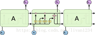
五、LSTM & GRU

基本LSTM

tensorflow提供了LSTM实现的一个basic版本，不包含lstm的一些高级扩展，同时也提供了一个标准接口，其中包含了lstm的扩展。分别为：tf.nn.rnn_cell.BasicLSTMCell(), tf.nn.rnn_cell.LSTMCell()

LSTM的结构

盗用一下Understanding LSTM Networks上的图 

图一

 

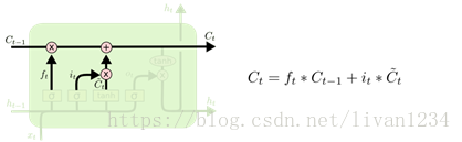
图二

 

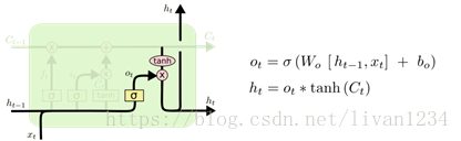
图三

tensorflow中的BasicLSTMCell()是完全按照这个结构进行设计的

    #tf.nn.rnn_cell.BasicLSTMCell(num_units,forget_bias, input_size, state_is_tupe=Flase, activation=tanh)

cell =tf.nn.rnn_cell.BasicLSTMCell(num_units, forget_bias=1.0, input_size=None,state_is_tupe=Flase, activation=tanh)

    #num_units:图一中ht的维数，如果num_units=10,那么ht就是10维行向量

    #forget_bias：还不清楚这个是干嘛的

    #input_size:[batch_size,max_time, size]。假设要输入一句话，这句话的长度是不固定的，max_time就代表最长的那句话是多长，size表示你打算用多长的向量代表一个word，即embedding_size（embedding_size和size的值不一定要一样）

    #state_is_tuple:true的话，返回的状态是一个tuple:(c=array([[]]), h=array([[]]):其中c代表Ct的最后时间的输出，h代表Ht最后时间的输出，h是等于最后一个时间的output的

    #图三向上指的ht称为output

    #此函数返回一个lstm_cell，即图一中的一个A

如果你想要设计一个多层的LSTM网络，你就会用到tf.nn.rnn_cell.MultiRNNCell(cells, state_is_tuple=False),这里多层的意思上向上堆叠，而不是按时间展开

lstm_cell = tf.nn.rnn_cell.MultiRNNCells(cells,state_is_tuple=False)

    #cells:一个cell列表，将列表中的cell一个个堆叠起来，如果使用cells=[cell]*4的话，就是四曾，每层cell输入输出结构相同

    #如果state_is_tuple:则返回的是 n-tuple，其中n=len(cells): tuple:(c=[batch_size, num_units],h=[batch_size,num_units])

这是，网络已经搭好了，tensorflow提供了一个非常方便的方法来生成初始化网络的state

initial_state =lstm_cell.zero_state(batch_size, dtype=)

    #返回[batch_size, 2*len(cells)],或者[batch_size, s]

    #这个函数只是用来生成初始化值的

现在进行时间展开，有两种方法： 
法一： 
使用现成的接口：

tf.nn.dynamic_rnn(cell, inputs,sequence_length=None, initial_state=None,dtype=None,time_major=False)

    #此函数会通过，inputs中的max_time将网络按时间展开

    #cell:将上面的lstm_cell传入就可以

    #inputs:[batch_size,max_time, size]如果time_major=Flase. [max_time,batch_size, size]如果time_major=True

    #sequence_length:是一个list，如果你要输入三句话，且三句话的长度分别是5,10,25,那么sequence_length=[5,10,25]

    #返回：（outputs, states）:output，[batch_size, max_time, num_units]如果time_major=False。 [max_time,batch_size,num_units]如果time_major=True。states:[batch_size, 2*len(cells)]或[batch_size,s]

    #outputs输出的是最上面一层的输出，states保存的是最后一个时间输出的states

法二

outputs = []

states = initial_states

with tf.variable_scope("RNN"):

    fortime_step in range(max_time):

       if time_step>0:tf.get_variable_scope().reuse_variables()#LSTM同一曾参数共享，

       (cell_out, state) = lstm_cell(inputs[:,time_step,:], state)

       outputs.append(cell_out)

已经得到输出了，就可以计算loss了,根据你自己的训练目的确定loss函数

GRU

GRU结构图 
来自Understanding LSTM Networks 

图四

tenforflow提供了tf.nn.rnn_cell.GRUCell()构建一个GRU单元

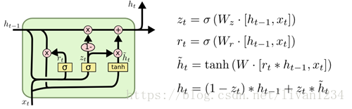
cell = tenforflow提供了tf.nn.rnn_cell.GRUCell(num_units, input_size=None, activation=tanh)

#参考lstm cell 使用

六、常用方法补充：

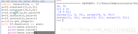
tf.unstack()

　　将给定的R维张量拆分成R-1维张量

　　将value根据axis分解成num个张量，返回的值是list类型，如果没有指定num则根据axis推断出！

DEMO：

1 2 3 4 5 6 7 8 9 10 11 12 13

import tensorflow as tf a = tf.constant([3,2,4,5,6]) b = tf.constant([1,6,7,8,0]) c = tf.stack([a,b],axis=0) d = tf.stack([a,b],axis=1) e = tf.unstack([a,b],axis=0) f = tf.unstack([a,b],axis=1)   with tf.Session() as sess:     print(sess.run(c))     print(sess.run(d))     print(sess.run(e))     print(sess.run(f))

输出：

[[3 2 4 5 6]
[1 6 7 8 0]]

--------------------
[[3 1]
[2 6]
[4 7]
[5 8]
[6 0]]

----------------------
[array([3, 2, 4, 5, 6]), array([1, 6, 7, 8, 0])]

----------------------
[array([3, 1]), array([2, 6]), array([4, 7]), array([5, 8]), array([6, 0])]

七、tf.nn.softmax_cross_entropy_with_logits的用法：

在计算loss的时候，最常见的一句话就是tf.nn.softmax_cross_entropy_with_logits，那么它到底是怎么做的呢？

首先明确一点，loss是代价值，也就是我们要最小化的值.

tf.nn.softmax_cross_entropy_with_logits(logits,labels, name=None)

除去name参数用以指定该操作的name，与方法有关的一共两个参数：

第一个参数logits：就是神经网络最后一层的输出，如果有batch的话，它的大小就是[batchsize，num_classes]，单样本的话，大小就是num_classes

第二个参数labels：实际的标签，大小同上

具体的执行流程大概分为两步：

第一步是先对网络最后一层的输出做一个softmax，这一步通常是求取输出属于某一类的概率，对于单样本而言，输出就是一个num_classes大小的向量（[Y1，Y2,Y3...]其中Y1，Y2，Y3...分别代表了是属于该类的概率）

至于为什么是用的这个公式？这里不介绍了，涉及到比较多的理论证明

第二步是softmax的输出向量[Y1，Y2,Y3...]和样本的实际标签做一个交叉熵，公式如下：

其中,指代实际的标签中第i个的值（用mnist数据举例，如果是3，那么标签是[0，0，0，1，0，0，0，0，0，0]，除了第4个值为1，其他全为0）

就是softmax的输出向量[Y1，Y2,Y3...]中，第i个元素的值

显而易见，预测越准确，结果的值越小（别忘了前面还有负号），最后求一个平均，得到我们想要的loss

注意！！！这个函数的返回值并不是一个数，而是一个向量，如果要求交叉熵，我们要再做一步tf.reduce_sum操作,就是对向量里面所有元素求和，最后才得到   ，如果求loss，则要做一步tf.reduce_mean操作，对向量求均值！

最后上代码:

import tensorflow as tf 

#our NN's output 

logits=tf.constant([[1.0,2.0,3.0],[1.0,2.0,3.0],[1.0,2.0,3.0]]) 

#step1:do softmax 

y=tf.nn.softmax(logits) 

#true label 

y_=tf.constant([[0.0,0.0,1.0],[0.0,0.0,1.0],[0.0,0.0,1.0]]) 

#step2:do cross_entropy 

cross_entropy =-tf.reduce_sum(y_*tf.log(y)) 

#do cross_entropy just one step 

cross_entropy2=tf.reduce_sum(tf.nn.softmax_cross_entropy_with_logits(logits,y_))#dont forget tf.reduce_sum()!! 

 

with tf.Session() as sess: 

   softmax=sess.run(y) 

   c_e = sess.run(cross_entropy) 

   c_e2 = sess.run(cross_entropy2) 

   print("step1:softmax result=") 

   print(softmax) 

   print("step2:cross_entropy result=") 

   print(c_e) 

   print("Function(softmax_cross_entropy_with_logits)result=") 

   print(c_e2) 

 

输出结果是：

 

step1:softmax result= 

[[ 0.09003057  0.24472848 0.66524094] 

 [0.09003057  0.24472848  0.66524094] 

 [0.09003057  0.24472848  0.66524094]] 

step2:cross_entropy result= 

1.22282 

Function(softmax_cross_entropy_with_logits)result= 

1.2228 

 

最后大家可以试试e^1/(e^1+e^2+e^3)是不是0.09003057，发现确实一样！！这也证明了我们的输出是符合公式逻辑的

 

八、RNN应用：

Ø  RNN案例（一）

# -*- coding: utf-8 -*-

import tensorflow as tf

importtensorflow.examples.tutorials.mnist.input_data as input_data

mnist =input_data.read_data_sets("MNIST_data/", one_hot=True)    

lr = 0.001

training_iters = 100000

batch_size = 128

n_inputs = 28

n_steps = 28

n_hidden_units = 128

n_classes = 10

# 生成两个占位符；

x = tf.placeholder(tf.float32, [None,n_steps, n_inputs])

y = tf.placeholder(tf.float32, [None,n_classes])

weights = {

    # 随机生成一个符合正态图形的矩阵，作为in和out的初始值。

   'in':tf.Variable(tf.random_normal([n_inputs, n_hidden_units])),

   'out':tf.Variable(tf.random_normal(n_hidden_units, n_classes)),

    }

 

biases = {

   'in':tf.Variable(tf.constant(0.1, shape=[n_hidden_units, ])),

   'out':tf.Variable(tf.constant(0.1, shape=[n_classes, ])),

    }

def RNN(X, weights, biases):

    # 第一步：输入的x为三维数据，因此需要进行相应的维度变换；转换成2维，然后与w、b进行交易，运算完成后，再将x转换成三维；

   X=tf.reshape(X, [-1, n_inputs])

   X_in = tf.matmul(X, weights['in'])+biases['in']

   X_in = tf.reshape(X_in, [-1, n_steps, n_hidden_units])

   

    # 第二步：即构建cell的初始值，并进行建模运算；

    #n_hidden_units:是ht的维数，表示128维行向量；state_is_tuple表示tuple形式，返回一个lstm的单元，即一个ht。

   lstm_cell = tf.contrib.rnn.BasicLSTMCell(n_hidden_units,forget_bias=1.0, state_is_tuple=True)

    # 将LSTM的状态初始化全为0数组，batch_size给出一个batch大小。

   init_state = lstm_cell.zero_state(batch_size, dtype=tf.float32)

    # 运算一个神经单元的输出值与状态，动态构建RNN模型，在这个模型中实现ht与x的结合。

   outputs, final_state = tf.nn.dynamic_rnn(lstm_cell, X_in,initial_state=init_state, time_major=False)

   

    # 第三步：将输出值进行格式转换，然后运算输出，即可。

    # 矩阵的转置，[0,1,2]为正常顺序[高，长，列]，想要更换哪个就更换哪个的顺序即可,并实现矩阵解析。

   outputs = tf.unstack(tf.transpose(outputs, [1,0,2]))

   results = tf.matmul(outputs[-1], weights['out']) + biases['out']

   return results

# 创建一个模型，然后进行测试。

pred = RNN(x, weights, biases)

# softmax_cross_entropy_with_logits：将神经网络最后一层的输出值pred与实际标签y作比较，然后计算全局平均值，即为损失。

cost =tf.reduce_mean(tf.nn.softmax_cross_entropy_with_logits(pred, y))

# 用梯度下降优化，下降速率为0.001。

train_op =tf.train.AdamOptimizer(lr).minimize(cost)

# 计算准确度。

correct_pred = tf.equal(tf.argmax(pred, 1),tf.argmax(y, 1))

accuracy =tf.reduce_mean(tf.cast(correct_pred, tf.float32))

init = tf.global_variables_initializer()

with tf.Session() as sess:

   sess.run(init)

   step = 0

   while step*batch_size < training_iters:

       batch_xs, batch_ys = mnist.train.next_batch(batch_size)

       batch_xs = batch_xs.reshape([batch_size, n_steps, n_inputs])

       sess.run([train_op], feed_dict={

           x:batch_xs,

           y:batch_ys,

           })

        if step % 20 ==0:

           print(sess.run(accuracy, feed_dict={

                x:batch_xs,

                y:batch_ys,

                }))

           step += 1

 

 

Ø  RNN案例（二）

# num_epochs = 100   

# total_series_length = 50000   

# truncated_backprop_length = 15   

# state_size = 4   

# num_classes = 2   

# echo_step = 3   

# batch_size = 5   

# num_batches =total_series_length//batch_size//truncated_backprop_length   

#

# def generateData():   

#     x= np.array(np.random.choice(2, total_series_length, p=[0.5, 0.5]))   

#     y= np.roll(x, echo_step)   

#    y[0:echo_step] = 0   

#    

#     x= x.reshape((batch_size, -1))  # Thefirst index changing slowest, subseries as rows   

#     y= y.reshape((batch_size, -1))   

#    

#    return (x, y)   

#

# batchX_placeholder =tf.placeholder(tf.float32, [batch_size, truncated_backprop_length])   

# batchY_placeholder =tf.placeholder(tf.int32, [batch_size, truncated_backprop_length])   

#

# init_state = tf.placeholder(tf.float32,[batch_size, state_size])   

#

# W =tf.Variable(np.random.rand(state_size+1, state_size), dtype=tf.float32)   

# b = tf.Variable(np.zeros((1,state_size)),dtype=tf.float32)   

#

# W2 = tf.Variable(np.random.rand(state_size,num_classes),dtype=tf.float32)   

# b2 = tf.Variable(np.zeros((1,num_classes)),dtype=tf.float32)   

#

# # Unpack columns   

# inputs_series =tf.unstack(batchX_placeholder, axis=1)   

# labels_series =tf.unstack(batchY_placeholder, axis=1)   

#

# # Forward pass   

# current_state = init_state   

# states_series = []   

# for current_input in inputs_series:   

#    current_input = tf.reshape(current_input, [batch_size, 1])   

#    input_and_state_concatenated = tf.concat(1, [current_input,current_state])  # Increasing number ofcolumns   

#

#    next_state = tf.tanh(tf.matmul(input_and_state_concatenated, W) +b)  # Broadcasted addition   

#    states_series.append(next_state)   

#    current_state = next_state   

#

# logits_series = [tf.matmul(state, W2) + b2for state in states_series] #Broadcasted addition   

# predictions_series = [tf.nn.softmax(logits)for logits in logits_series]   

#

# losses =[tf.nn.sparse_softmax_cross_entropy_with_logits(logits, labels) for logits,labels in zip(logits_series,labels_series)]   

# total_loss = tf.reduce_mean(losses)   

#

# train_step =tf.train.AdagradOptimizer(0.3).minimize(total_loss)   

# def plot(loss_list, predictions_series,batchX, batchY):   

#    plt.subplot(2, 3, 1)   

#    plt.cla()   

#    plt.plot(loss_list)   

#

#    for batch_series_idx in range(5):   

#        one_hot_output_series = np.array(predictions_series)[:, batch_series_idx,:]   

#        single_output_series = np.array([(1 if out[0] < 0.5 else 0) for outin one_hot_output_series])   

#        

#        plt.subplot(2, 3, batch_series_idx + 2)   

#        plt.cla()   

#        plt.axis([0, truncated_backprop_length, 0, 2])   

#        left_offset = range(truncated_backprop_length)   

#        plt.bar(left_offset, batchX[batch_series_idx, :], width=1,color="blue")   

#        plt.bar(left_offset, batchY[batch_series_idx, :] * 0.5, width=1,color="red")   

#        plt.bar(left_offset, single_output_series * 0.3, width=1,color="green")   

#

#    plt.draw()   

#    plt.pause(0.0001)   

#

# with tf.Session() as sess:   

#    sess.run(tf.initialize_all_variables())   

#    plt.ion()   

#    plt.figure()   

#    plt.show()   

#    loss_list = []   

#

# for epoch_idx in range(num_epochs):   

#    x,y = generateData()   

#    _current_state = np.zeros((batch_size, state_size))   

#    print("New data, epoch", epoch_idx)   

#

# for batch_idx in range(num_batches):   

#    start_idx = batch_idx * truncated_backprop_length   

#    end_idx = start_idx + truncated_backprop_length   

#    

#    batchX = x[:,start_idx:end_idx]   

#    batchY = y[:,start_idx:end_idx]   

#

#    _total_loss, _train_step, _current_state, _predictions_series =sess.run(   

#    [total_loss, train_step, current_state, predictions_series],   

#    feed_dict={   

#    batchX_placeholder:batchX,   

#    batchY_placeholder:batchY,   

#     init_state:_current_state   

#    })   

#    loss_list.append(_total_loss)   

#    if batch_idx%100 == 0:   

#        print("Step",batch_idx, "Loss", _total_loss)   

#        plot(loss_list, _predictions_series, batchX, batchY)   

#    plt.ioff()   

#    plt.show()

 

 

Ø  LSTM_RNN案例（三）：

# -*-coding: utf-8 -*- 

import numpy as np   

import tensorflow as tf   

import matplotlib.pyplot as plt   

from asn1crypto._ffi import null

BATCH_START=0     #建立batch data的时候的index

TIME_STEPS=20     #backpropagation throughtime的time_steps

BATCH_SIZE=50     #

INPUT_SIZE=1      #sin数据输入size

OUTPUT_SIZE=1     #cos数据输入size

CELL_SIZE=10      #RNN的hiden unit size

LR=0.006         #学习率

# 定义一个生成数据的get_batch的function：

def get_batch():

    global BATCH_START, TIME_STEPS

    xs=np.arange(BATCH_START,BATCH_START+TIME_STEPS*BATCH_SIZE)

        .reshape((BATCH_SIZE,TIME_STEPS))/(10*np.pi)

    seq=np.sin(xs)

    res=np.cos(xs)

    BATCH_START+=TIME_STEPS

    # np.newaxis:在功能上等价于none；

    return [seq[:,:,np.newaxis],res[:,:,np.newaxis],xs]

class LSTMRNN(object):

    def __init__(self, n_steps, input_size, output_size, cell_size,batch_size):

        self.n_steps=n_steps

        self.input_size=input_size

        self.output_size=output_size

        self.cell_size=cell_size

        self.batch_size=batch_size

        # 构建命名空间，在inputs命名空间下的xs和ys与其他空间下的xs和ys是不冲突的，一般与variable一起用。

        with tf.name_scope('inputs'):

            self.xs=tf.placeholder(tf.float32,[None, n_steps, input_size], name='xs')

            self.ys=tf.placeholder(tf.float32,[None, n_steps, output_size], name='ys')

        # variable_scope与get_variable()一起用，实现变量共享，指向同一个内存空间。       

      with tf.variable_scope('in_hidden'):

            self.add_input_layer()

        with tf.variable_scope('LSTM_cell'):

            self.add_cell()

        with tf.variable_scope('out_hidden'):

            self.add_output_layer()

        with tf.name_scope('cost'):

            self.compute_cost()

        with tf.name_scope('train'):

            self.train_op=tf.train.AdamOptimizer(LR).minimize(self.cost)

    def add_input_layer(self,):

        l_in_x = tf.reshape(self.xs, [-1, self.input_size], name='2_2D')

        Ws_in=self._weight_variable([self.input_size, self.cell_size])

        bs_in=self._bias_variable([self.cell_size,])

        with tf.name_scope('Wx_plus_b'):

            l_in_y=tf.matmul(l_in_x,Ws_in)+bs_in

        self.l_in_y=tf.reshape(l_in_y,[-1, self.n_steps, self.cell_size],name='2_3D')

       

    def add_cell(self):

        lstm_cell=tf.contrib.rnn.BasicLSTMCell(self.cell_size,forget_bias=1.0, state_is_tuple=True)

        with tf.name_scope('initial_state'):

            self.cell_init_state=lstm_cell.zero_state(self.batch_size,dtype=tf.float32)

        self.cell_outputs,self.cell_final_state=tf.nn.dynamic_rnn(lstm_cell, self.l_in_y,initial_state=self.cell_init_state, time_major=False)

    def add_output_layer(self):

        l_out_x=tf.reshape(self.cell_outputs,[-1, self.cell_size], name='2_2D')

        Ws_out=self._weight_variable([self.cell_size,self.output_size])

        bs_out=self._bias_variable([self.output_size,])

        with tf.name_scope('Wx_plus_b'):

            self.pred=tf.matmul(l_out_x,Ws_out)+bs_out

    # 求交叉熵

    def compute_cost(self):

       losses=tf.contrib.legacy_seq2seq.sequence_loss_by_example(

            [tf.reshape(self.pred, [-1], name='reshape_pred')],

            [tf.reshape(self.ys, [-1], name='reshape_target')],

            [tf.ones([self.batch_size*self.n_steps],dtype=tf.float32)],

            average_across_timesteps=True,

            softmax_loss_function=self.ms_error,

            name='losses'

            )

        with tf.name_scope('average_cost'):

            self.cost=tf.div(

                tf.reduce_sum(losses, name='losses_sum'),

                self.batch_size,

                name='average_cost',

            )

            tf.summary.scalar('cost',self.cost)

    def ms_error(self,labels,logits):

        #求方差

        return tf.square(tf.subtract(labels,logits))

    def _weight_variable(self, shape, name='weights'):

       initializer=tf.random_normal_initializer(mean=0, stddev=1.,)

        return tf.get_variable(shape=shape,initializer=initializer, name=name)

    def _bias_variable(self, shape, name='biases'):

        initializer=tf.constant_initializer(0, 1)

        return tf.get_variable(name=name, shape=shape,initializer=initializer)   

if __name__=='__main__':

    model=LSTMRNN(TIME_STEPS, INPUT_SIZE,OUTPUT_SIZE, CELL_SIZE, BATCH_SIZE)

    sess=tf.Session()

    sess.run(tf.global_variables_initializer())

    state=null

    for i in range(200):

        seq, res, xs=get_batch()

        if i == 0:

            feed_dict={

                model.xs:seq,

                model.ys:res,

                }

        else:

            feed_dict={

                model.xs:seq,

                model.ys:res,

                model.cell_init_state:state

                }

        _, cost, state, pred=sess.run(

            [model.train_op, model.cost,model.cell_final_state, model.pred],

            feed_dict=feed_dict)

        if i%20==0:

            print('cost:',round(cost, 4))

九、使用flags定义命令行参数

import tensorflow as tf

第一个是参数名称，第二个参数是默认值，第三个是参数描述

tf.app.flags.DEFINE_string('str_name', 'def_v_1',"descrip1")

tf.app.flags.DEFINE_integer('int_name', 10,"descript2")

tf.app.flags.DEFINE_boolean('bool_name', False, "descript3")

 

FLAGS = tf.app.flags.FLAGS

 

#必须带参数，否则：'TypeError: main() takes no arguments (1given)';   main的参数名随意定义，无要求

defmain(_):

    # 在这个函数中添加脚本所需要处理的内容。

    print(FLAGS.str_name)

    print(FLAGS.int_name)

    print(FLAGS.bool_name)

 

if __name__ == '__main__':

   tf.app.run()  #执行main函数

注：

FLAGS命令是指编写一个脚本文件，在执行这个脚本时添加相应的参数；

如（上面文件叫tt.py）：

python tt.py --str_name test_str--int_name 99 --bool_name True

 

十、tensor变换：

#对于2-D

# Tensor变换主要是对矩阵进行相应的运算工作，包涵的方法主要有：reduce_……（a, axis）系列；如果不加axis的话都是针对整个矩阵进行运算。

tf.reduce_sum(a, 1）#对axis1

tf.reduce_mean(a,0) #每列均值

第二个参数是axis，如果为0的话，res[i]=∑ja[j,i]res[i]=∑ja[j,i]即（res[i]=∑a[:,i]res[i]=∑a[:,i]）， 如果是1的话，res[i]=∑ja[i,j]res[i]=∑ja[i,j] 
NOTE:返回的都是行向量,（axis等于几，就是对那维操作,i.e.:沿着那维操作, 其它维度保留）

#关于concat，可以用来进行降维 3D->2D , 2D->1D

tf.concat(concat_dim, data)

#arr = np.zeros([2,3,4,5,6])

In [6]: arr2.shape

Out[6]: (2, 3, 4, 5)

In [7]: np.concatenate(arr2, 0).shape

Out[7]: (6, 4, 5)   :(2*3, 4, 5)

In [9]: np.concatenate(arr2, 1).shape

Out[9]: (3, 8, 5)   :(3, 2*4, 5)

#tf.concat()

t1 = [[1, 2, 3], [4, 5, 6]]

t2 = [[7, 8, 9], [10, 11, 12]]

# 将t1, t2进行concat，axis为0，等价于将shape=[2,2, 3]的Tensor concat成

#shape=[4, 3]的tensor。在新生成的Tensor中tensor[:2,:]代表之前的t1

#tensor[2:,:]是之前的t2

tf.concat(0, [t1, t2]) ==> [[1, 2, 3], [4, 5, 6], [7, 8, 9], [10, 11, 12]]

 

# 将t1, t2进行concat，axis为1，等价于将shape=[2,2, 3]的Tensor concat成

#shape=[2, 6]的tensor。在新生成的Tensor中tensor[:,:3]代表之前的t1

#tensor[:,3:]是之前的t2

tf.concat(1, [t1, t2]) ==> [[1, 2, 3, 7, 8, 9], [4, 5, 6, 10, 11, 12]]

concat是将list中的向量给连接起来，axis表示将那维的数据连接起来，而其他维的结构保持不变

#squeeze 降维维度为1的降掉

tf.squeeze(arr, [])

降维，将维度为1的降掉

arr = tf.Variable(tf.truncated_normal([3,4,1,6,1], stddev=0.1))

arr2 = tf.squeeze(arr, [2,4])

arr3 = tf.squeeze(arr) #降掉所以是1的维

 

# split(dimension, num_split, input)：dimension的意思就是输入张量的哪一个维度，如果是0就表示对第0维度进行切割。num_split就是切割的数量，如果是2就表示输入张量被切成2份，每一份是一个列表。

tf.split(split_dim, num_split, value, name='split')

# 'value' is a tensor with shape [5, 30]

# Split 'value' into 3 tensors along dimension 1

split0, split1, split2 = tf.split(1, 3, value)

tf.shape(split0) ==> [5, 10]

 

#embedding: embedding_lookup是按照向量获取矩阵中的值，[0,2,3,1]是取第0,2,3,1个向量。

mat = np.array([1,2,3,4,5,6,7,8,9]).reshape((3,-1))

ids = [[1,2], [0,1]]

res = tf.nn.embedding_lookup(mat, ids)

res.eval()

array([[[4, 5, 6],

        [7, 8, 9]],

       [[1, 2, 3],

        [4, 5, 6]]])

# expand_dims：扩展维度，如果想用广播特性的话，经常会用到这个函数

# 't' is a tensor of shape [2]

#一次扩展一维

shape(tf.expand_dims(t, 0)) ==> [1, 2]

shape(tf.expand_dims(t, 1)) ==> [2, 1]

shape(tf.expand_dims(t, -1)) ==> [2, 1]

# 't2' is a tensor of shape [2, 3, 5]

shape(tf.expand_dims(t2, 0)) ==> [1, 2, 3, 5]

shape(tf.expand_dims(t2, 2)) ==> [2, 3, 1, 5]

shape(tf.expand_dims(t2, 3)) ==> [2, 3, 5, 1]

tf.slice()

tf.slice(input_, begin, size, name=None) 
这个函数的作用是从输入数据input中提取出一块切片

o   切片的尺寸是size，切片的开始位置是begin。

o   切片的尺寸size表示输出tensor的数据维度，其中size[i]表示在第i维度上面的元素个数。

o   开始位置begin表示切片相对于输入数据input_的每一个偏移量

import tensorflow as tf

import numpy as np

sess = tf.Session()

input=tf.constant([[[1, 1, 1], [2, 2, 2]], [[3, 3, 3], [4, 4, 4]], [[5, 5, 5], [6, 6, 6]]])

data = tf.slice(input, [1, 0, 0], [1, 1, 3])

print(sess.run(data))

"""[1,0,0]表示第一维偏移了1 则是从[[[3, 3, 3],[4, 4, 4]],[[5, 5, 5], [6, 6, 6]]]中选取数据然后选取第一维的第一个，第二维的第一个数据，第三维的三个数据"""

# [[[3 3 3]]]

#array([[ 6,  7],

#       [11, 12]])

理解tf.slice()最好是从返回值上去理解，现在假设input的shape是[a1, a2, a3], begin的值是[b1, b2, b3],size的值是[s1, s2, s3],那么tf.slice()返回的值就是 input[b1:b1+s1,b2:b2+s2, b3:b3+s3]。 
如果 si=−1si=−1 ，那么 返回值就是 input[b1:b1+s1,...,bi: ,...]

注意：input[1:2] 取不到input[2]

tf.stack()

tf.stack(values, axis=0, name=’stack’)

tf.stack（）这是一个矩阵拼接的函数，tf.unstack（）则是一个矩阵分解的函数

将 a list of R 维的Tensor堆成 R+1维的Tensor。 
Given a list of length N of tensors of shape (A, B, C); 
if axis == 0 then the output tensor will have the shape (N, A, B, C)

这时 res[i,:,:,:] 就是原 list中的第 i 个 tensor

if axis == 1 thenthe output tensor will have the shape (A, N, B, C).

这时 res[:,i,:,:] 就是原list中的第 i 个 tensor

Etc.

# 'x' is [1, 4]

# 'y' is [2, 5]

# 'z' is [3, 6]

stack([x, y, z]) => [[1, 4], [2, 5], [3, 6]]  # Pack along first dim.

stack([x, y, z], axis=1) => [[1, 2, 3], [4, 5, 6]]

tf.gather()：按照指定的下标集合从axis=0中抽取子集

tf.gather(params, indices, validate_indices=None,name=None)

·        tf.slice(input_,begin, size, name=None)：按照指定的下标范围抽取连续区域的子集

·        tf.gather(params,indices, validate_indices=None, name=None)：按照指定的下标集合从axis=0中抽取子集，适合抽取不连续区域的子集

input = [[[1, 1, 1], [2, 2, 2]],

         [[3, 3, 3], [4, 4, 4]],

         [[5, 5, 5], [6, 6, 6]]]

tf.slice(input, [1, 0, 0], [1, 1, 3]) ==> [[[3, 3, 3]]]

tf.slice(input, [1, 0, 0], [1, 2, 3]) ==> [[[3, 3, 3],

                                            [4, 4, 4]]]

tf.slice(input, [1, 0, 0], [2, 1, 3]) ==> [[[3, 3, 3]],

                                           [[5, 5, 5]]]

tf.gather(input, [0, 2]) ==> [[[1, 1, 1], [2, 2, 2]],

                              [[5, 5, 5], [6, 6, 6]]]

indices must be an integer tensor of any dimension(usually 0-D or 1-D).

Produces an output tensor with shape indices.shape +params.shape[1:]

# Scalar indices, 会降维

output[:, ..., :] = params[indices, :, ... :]

# Vector indices

output[i, :, ..., :] = params[indices[i], :, ... :]

# Higher rank indices，会升维

output[i, ..., j, :, ... :] = params[indices[i, ..., j],:, ..., :]

tf.pad

tf.pad(tensor, paddings, mode="CONSTANT", name=None)

·        tensor: 任意shape的tensor，维度 Dn

·        paddings: [Dn, 2] 的 Tensor, Padding后tensor的某维上的长度变为padding[D,0]+tensor.dim_size(D)+padding[D,1]

·        mode: CONSTANT表示填0, REFLECT表示反射填充,SYMMETRIC表示对称填充。

·        函数原型： 
tf.pad 
pad(tensor, paddings, mode=’CONSTANT’, name=None)

（输入数据，填充的模式，填充的内容，名称）

·        这里紧紧解释paddings的含义： 
它是一个Nx2的列表， 
在输入维度n上，则paddings[n,0] 表示该维度内容前面加0的个数, 如对矩阵来说，就是行的最上面或列最左边加几排0 
paddings[n, 1] 表示该维度内容后加0的个数。

·        举个例子： 
输入 tensor 形如 
[[ 1, 2], 
[1, 2]] 
而paddings = [[1, 1], [1, 1]] （[[上，下],[左，右]]）

Tensor=[[1,2],[1,2]]

Paddings=[[1,1],[1,1]]

Init=tf.global_variables_initializer()

Withtf.Session() as sess:

Sess.run(init)

Print(sess.run(tf.pad(tensor,paddings, mode=’CONSTANT’)))
则结果为:

[[0, 0, 0, 0], 
[0, 1, 2, 0], 
[0, 1, 2, 0], 
[0, 0, 0, 0]]

十一、损失函数：

损失函数的运算规则：

tf.nn.softmax_cross_entropy_with_logits(logits, labels, name=None)

除去name参数用以指定该操作的name，与方法有关的一共两个参数：

第一个参数logits：就是神经网络最后一层的输出，如果有batch的话，它的大小就是[batchsize，num_classes]，单样本的话，大小就是num_classes

第二个参数labels：实际的标签，大小同上

具体的执行流程大概分为两步：

第一步是先对网络最后一层的输出做一个softmax，这一步通常是求取输出属于某一类的概率，对于单样本而言，输出就是一个num_classes大小的向量（[Y1，Y2,Y3...]其中Y1，Y2，Y3...分别代表了是属于该类的概率）。

第二步是softmax的输出向量[Y1，Y2,Y3...]和样本的实际标签做一个交叉熵。

第三步是求一个平均，得到我们想要的loss

最后上代码:

import tensorflow as tf  

#our NN's output  

logits=tf.constant([[1.0,2.0,3.0],[1.0,2.0,3.0],[1.0,2.0,3.0]])  

#step1:do softmax  

y=tf.nn.softmax(logits)  

#true label  

y_=tf.constant([[0.0,0.0,1.0],[0.0,0.0,1.0],[0.0,0.0,1.0]])  

#step2:do cross_entropy  

cross_entropy = -tf.reduce_sum(y_*tf.log(y))  

#do cross_entropy just one step  

cross_entropy2=tf.reduce_sum(tf.nn.softmax_cross_entropy_with_logits(logits, y_))#dont forget tf.reduce_sum()!!  

with tf.Session() as sess:  

    softmax=sess.run(y)  

    c_e = sess.run(cross_entropy)  

    c_e2 = sess.run(cross_entropy2)  

    print("step1:softmax result=")  

    print(softmax)  

    print("step2:cross_entropy result=")  

    print(c_e)  

    print("Function(softmax_cross_entropy_with_logits) result=")  

    print(c_e2)  

输出结果是：

step1:softmax result=  

[[ 0.09003057  0.24472848  0.66524094]  

 [ 0.09003057  0.24472848  0.66524094]  

 [ 0.09003057  0.24472848  0.66524094]]  

step2:cross_entropy result=  1.22282  

Function(softmax_cross_entropy_with_logits) result=  1.2228  

交叉熵可在神经网络(机器学习)中作为损失函数，p表示真实标记的分布，q则为训练后的模型的预测标记分布，交叉熵损失函数可以衡量p与q的相似性。交叉熵作为损失函数还有一个好处是使用sigmoid函数在梯度下降时能避免均方误差损失函数学习速率降低的问题，因为学习速率可以被输出的误差所控制。tensorflow中自带的函数可以轻松的实现交叉熵的计算。

tf.nn.softmax_cross_entropy_with_logits(_sentinel=None, labels=None, logits=None, dim=-1, name=None)

Computes softmax cross entropy between logits and labels.

注意：如果labels的每一行是one-hot表示，也就是只有一个地方为1，其他地方为0，可以使用tf.sparse_softmax_cross_entropy_with_logits()

警告：

1. 这个操作的输入logits是未经缩放的，该操作内部会对logits使用softmax操作

2. 参数labels,logits必须有相同的形状 [batch_size, num_classes] 和相同的类型(float16, float32, float64)中的一种

参数：

_sentinel: 一般不使用

labels: labels的每一行labels[i]必须为一个概率分布

logits: 未缩放的对数概率

dims: 类的维度，默认-1，也就是最后一维

name: 该操作的名称

返回值：长度为batch_size的一维Tensor

下面用个小例子来看看该函数的用法

import tensorflow as tf

labels = [[0.2,0.3,0.5],

          [0.1,0.6,0.3]]

logits = [[2,0.5,1],

          [0.1,1,3]]

logits_scaled = tf.nn.softmax(logits)

result1 = tf.nn.softmax_cross_entropy_with_logits(labels=labels, logits=logits)

result2 = -tf.reduce_sum(labels*tf.log(logits_scaled),1)

result3 = tf.nn.softmax_cross_entropy_with_logits(labels=labels, logits=logits_scaled)

with tf.Session() as sess:

    print sess.run(result1)

    print sess.run(result2)

    print sess.run(result3)

>>>[ 1.41436887  1.66425455]

>>>[ 1.41436887  1.66425455]

>>>[ 1.17185783  1.17571414]

上述例子中，labels的每一行是一个概率分布，而logits未经缩放(每行加起来不为1)，我们用定义法计算得到交叉熵result2,和套用tf.nn.softmax_cross_entropy_with_logits()得到相同的结果, 但是将缩放后的logits_scaled输tf.nn.softmax_cross_entropy_with_logits(), 却得到错误的结果，所以一定要注意，这个操作的输入logits是未经缩放的

下面来看tf.nn.sparse_softmax_cross_entropy_with_logits(_sentinel=None, labels=None, logits=None, name=None)

这个函数与上一个函数十分类似，唯一的区别在于labels.

注意：

对于此操作，给定标签的概率被认为是排他的。labels的每一行为真实类别的索引

警告：

1. 这个操作的输入logits同样是是未经缩放的，该操作内部会对logits使用softmax操作

2. 参数logits的形状 [batch_size, num_classes] 和labels的形状[batch_size]

返回值：长度为batch_size的一维Tensor, 和label的形状相同，和logits的类型相同

import tensorflow as tf

labels = [0,2]

logits = [[2,0.5,1],

          [0.1,1,3]]

logits_scaled = tf.nn.softmax(logits)

result1 = tf.nn.sparse_softmax_cross_entropy_with_logits(labels=labels, logits=logits)

with tf.Session() as sess:

    print sess.run(result1)

>>>[ 0.46436879  0.17425454]

tf.nn.sparse_softmax_cross_entropy_with_logits(logits,labels, name=None)

def sparse_softmax_cross_entropy_with_logits(logits, labels, name=None):

#logits是最后一层的z（输入）

#A common use case is to have logits of shape `[batch_size, num_classes]` and

#labels of shape `[batch_size]`. But higher dimensions are supported.

#Each entry in `labels` must be an index in `[0, num_classes)`

#输出：loss [batch_size]

tf. nn.softmax_cross_entropy_with_logits(logits,targets, dim=-1, name=None)

def softmax_cross_entropy_with_logits(logits, targets, dim=-1, name=None):

#`logits` and `labels` must have the same shape `[batch_size, num_classes]`

#return loss:[batch_size], 里面保存是batch中每个样本的cross entropy

tf.nn.sigmoid_cross_entropy_with_logits(logits,targets, name=None)

def sigmoid_cross_entropy_with_logits(logits, targets, name=None):

#logits:[batch_size, num_classes],targets:[batch_size, size].logits作为用最后一层的输入就好，不需要进行sigmoid运算，函数内部进行了sigmoid操作。

#输出loss [batch_size, num_classes]。。。说的是logits，其实内部实现是relu

tf.nn.nce_loss(nce_weights,nce_biases, embed, train_labels, num_sampled, vocabulary_size)

def nce_loss(nce_weights, nce_biases, embed, train_labels, num_sampled, vocabulary_size):

#word2vec中用到了这个函数

#weights: A `Tensor` of shape `[num_classes, dim]`, or a list of `Tensor`

#        objects whose concatenation along dimension 0 has shape

#        [num_classes, dim].  The (possibly-partitioned) class embeddings.

#biases: A `Tensor` of shape `[num_classes]`.  The class biases.

#inputs: A `Tensor` of shape `[batch_size, dim]`.  The forward

#        activations of the input network.

#labels: A `Tensor` of type `int64` and shape `[batch_size,

#    num_true]`. The target classes.

#num_sampled: An `int`.  The number of classes to randomly sample per batch.

#num_classes: An `int`. The number of possible classes.

#num_true: An `int`.  The number of target classes per training example.

tf.nn.sequence_loss_by_example(logits,targets, weights, average_across_timesteps=True, softmax_loss_function=None,name=None):

def sequence_loss_by_example(logits, targets, weights,

                             average_across_timesteps=True,

                             softmax_loss_function=None, name=None):

#logits: List of 2D Tensors of shape [batch_size x num_decoder_symbols].

#targets: List of 1D batch-sized int32 Tensors of the same length as logits.

#weights: List of 1D batch-sized float-Tensors of the same length as logits.

#return:log_pers 形状是 [batch_size].

   for logit, target, weight in zip(logits, targets, weights):

      if softmax_loss_function is None:

        # TODO(irving,ebrevdo): This reshape is needed because

        # sequence_loss_by_example is called with scalars sometimes, which

        # violates our general scalar strictness policy.

        target = array_ops.reshape(target, [-1])

"""

变量声明，运算声明 例：w = tf.get_variable(name="vari_name", shape=[], dtype=tf.float32)

初始化op声明

"""

#创建saver对象，它添加了一些op用来save和restore模型参数

#后缀可加可不加

现在，训练好的模型参数已经存储好了，我们来看一下怎么调用训练好的参数 
变量保存的时候，保存的是 变量名：value，键值对。restore的时候，也是根据key-value来进行的(详见)

import tensorflow as tf

"""

变量声明，运算声明

初始化op声明

"""

#创建saver 对象

#想要实现这个功能的话,必须从Saver的构造函数下手

# Pass the variables as a dict:

saver = tf.train.Saver({'v1': v1, 'v2': v2})

# Or pass them as a list.

# Passing a list is equivalent to passing a dict with the variable op names

# as keys:

saver = tf.train.Saver({v.op.name: v for v in [v1, v2]})

#注意，如果不给Saver传var_list 参数的话， 他将已 所有可以保存的 variable作为其var_list的值。

这里使用了三种不同的方式来创建 saver 对象， 但是它们内部的原理是一样的。我们都知道，参数会保存到 checkpoint 文件中，通过键值对的形式在 checkpoint中存放着。如果 Saver 的构造函数中传的是 dict，那么在 save 的时候，checkpoint文件中存放的就是对应的 key-value。如下：

import tensorflow as tf

# Create some variables.

v1 = tf.Variable(1.0, name="v1")

v2 = tf.Variable(2.0, name="v2")

saver = tf.train.Saver({"variable_1":v1, "variable_2": v2})

# Use the saver object normally after that.

with tf.Session() as sess:

# 输出:

#tensor_name:  variable_1

#1.0

#tensor_name:  variable_2

#2.0

如果构建saver对象的时候，我们传入的是 list， 那么将会用对应 Variable 的 variable.op.name 作为 key。

import tensorflow as tf

# Create some variables.

v1 = tf.Variable(1.0, name="v1")

v2 = tf.Variable(2.0, name="v2")

# Use the saver object normally after that.

with tf.Session() as sess:

1.0

2.0

如果我们现在想将 checkpoint 中v2的值restore到v1 中，v1的值restore到v2中，我们该怎么做？ 
这时，我们只能采用基于 dict 的 saver

import tensorflow as tf

# Create some variables.

v1 = tf.Variable(1.0, name="v1")

v2 = tf.Variable(2.0, name="v2")

saver = tf.train.Saver({"variable_1":v1, "variable_2": v2})

# Use the saver object normally after that.

with tf.Session() as sess:

# Create some variables.

v1 = tf.Variable(1.0, name="v1")

v2 = tf.Variable(2.0, name="v2")

#restore的时候，variable_1对应到v2，variable_2对应到v1，就可以实现目的了。

saver = tf.train.Saver({"variable_1":v2, "variable_2": v1})

# Use the saver object normally after that.

with tf.Session() as sess:

# 输出的结果是 2.0 1.0，如我们所望

我们发现，其实 创建 saver对象时使用的键值对就是表达了一种对应关系：

·        save时，表示：variable的值应该保存到 checkpoint文件中的哪个 key下

·        restore时，表示：checkpoint文件中key对应的值，应该restore到哪个variable

其它

一个快速找到ckpt文件的方式

进行候选采样的时候，每次只评估所有类别的一个很小的子集，这样可以提高运算效率，在这样的方式下，计算函数的对应损失需要用到tf.sampled_softmax_loss()。

tf.sampled_softmax_loss()中调用了_compute_sampled_logits() 

#此函数和nce_loss是差不多的, 取样求loss

def sampled_softmax_loss(weights, #[num_classes, dim]

                           biases,  #[num_classes]

                           inputs,  #[batch_size, dim]

                           labels,  #[batch_size, num_true]

                           num_sampled,

                           num_classes,

                           num_true=1,

                         sampled_values=None,

                         remove_accidental_hits=True,

                         partition_strategy="mod",

                         name="sampled_softmax_loss"):

#return: [batch_size]

关于参数labels:一般情况下，num_true为1, labels的shpae为[batch_size, 1]。假设我们有1000个类别， 使用one_hot形式的label的话， 我们的labels的shape是[batch_size,num_classes]。显然，如果num_classes非常大的话，会影响计算性能。所以，这里采用了一个稀疏的方式,即：使用3代表了[0,0,0,1,0….]

Ø  tf.nn.seq2seq.embedding_attention_seq2seq（）

创建了input embedding matrix 和 output embedding matrix

def embedding_attention_seq2seq(encoder_inputs, #[T， batch_size]

                                decoder_inputs, #[out_T， batch_size]

                                cell,

                                num_encoder_symbols,

                                num_decoder_symbols,

                                embedding_size,

                                num_heads=1, #只采用一个read head

                                output_projection=None,

                                feed_previous=False,

                                dtype=None,

                                scope=None,

                                initial_state_attention=False):

#output_projection: (W, B) W:[output_size, num_decoder_symbols]

#B: [num_decoder_symbols]                    

(1)这个函数创建了一个inputs 的 embeddingmatrix. 
(2)计算了encoder的 output，并保存起来，用于计算attention

# Decoder.

  output_size = None

  if output_projection is None:

class EmbeddingWrapper(RNNCell):

  def __init__(self, cell, embedding_classes, embedding_size, initializer=None):

  def __call__(self, inputs, state, scope=None):#生成embedding矩阵[embedding_classes,embedding_size]

  #inputs: [batch_size, 1]

  #return : (output, state)

tf.nn.rnn_cell.OutputProgectionWrapper()

将rnn_cell的输出映射成想要的维度

class OutputProjectionWrapper(RNNCell):

  def __init__(self, cell, output_size): # output_size:映射后的size

  def __call__(self, inputs, state, scope=None):

#init 返回一个带output projection的 rnn_cell

tf.nn.seq2seq.embedding_attention_decoder()

#生成embedding matrix ：[num_symbols, embedding_size]

def embedding_attention_decoder(decoder_inputs, # T*batch_size

                                initial_state,

                                attention_states,

                                cell,

                                num_symbols,

                                embedding_size,

                                num_heads=1,

                                output_size=None,

                                output_projection=None,

                                feed_previous=False,

                                update_embedding_for_previous=True,

                                dtype=None,

                                scope=None,

                                initial_state_attention=False):

#核心代码

  embedding = variable_scope.get_variable("embedding",

                                          [num_symbols, embedding_size])  #output embedding

def attention_decoder(decoder_inputs, #[T, batch_size, input_size]

                      initial_state,  #[batch_size, cell.states]

                      attention_states, #[batch_size , attn_length , attn_size]

                      cell,

                      output_size=None,

                      num_heads=1,

                      loop_function=None,

                      dtype=None,

                      scope=None,

                      initial_state_attention=False):

论文中，在计算attention distribution的时候，提到了三个公式 

(1)uti=vT∗tanh(W1∗hi+W2∗dt)(1)uit=vT∗tanh(W1∗hi+W2∗dt)

 (2)sti=softmax(ati)(2)sit=softmax(ait)

 (3)d′=∑i=1TAsti∗hi(3)d′=∑i=1TAsit∗hi

其中，W1W1维度是[attn_vec_size, size], hihi:[size,1]，我们日常表示输入数据，都是用列向量表示，但是在tensorflow中，趋向用行向量表示。在这个函数中，为了计算 W1∗hiW1∗hi，使用了卷积的方式。

def rnn(cell, inputs, initial_state=None, dtype=None,

        sequence_length=None, scope=None):

#inputs: A length T list of inputs, each a `Tensor` of shape`[batch_size, input_size]`

#sequence_length: [batch_size], 指定sample 序列的长度

#return : (outputs, states), outputs: T*batch_size*output_size. states:batch_size*state

seq2seqModel

·        创建映射参数 proj_w, proj_b

·        声明：sampled_loss，看了word2vec的就会理解

·        声明：seq2seq_f()，构建了inputs的embedding和outputs的embedding，进行核心计算

·        使用model_with_buckets(),model_with_buckets中调用了seq2seq_f和 sampled_loss

model_with_buckets()

调用方法tf.nn.seq2seq.model_with_buckets()

def model_with_buckets(encoder_inputs, decoder_inputs, targets, weights,

                       buckets, seq2seq, softmax_loss_function=None,

                       per_example_loss=False, name=None):

"""Create a sequence-to-sequence model with support for bucketing.

The seq2seq argument is a function that defines a sequence-to-sequence model,

e.g., seq2seq = lambda x, y: basic_rnn_seq2seq(x, y, rnn_cell.GRUCell(24))

Args:

encoder_inputs: A list of Tensors to feed the encoder; first seq2seq input.

decoder_inputs: A list of Tensors to feed the decoder; second seq2seq input.

targets: A list of 1D batch-sized int32 Tensors (desired output sequence).

weights: List of 1D batch-sized float-Tensors to weight the targets.

buckets: A list of pairs of (input size, output size) for each bucket.

seq2seq: A sequence-to-sequence model function; it takes 2 input that agree with encoder_inputs and decoder_inputs, and returns a pair consisting of outputs and states (as, e.g., basic_rnn_seq2seq).

softmax_loss_function: Function (inputs-batch, labels-batch) -> loss-batch

to be used instead of the standard softmax (the default if this is None).

per_example_loss: Boolean. If set, the returned loss will be a batch-sized

tensor of losses for each sequence in the batch. If unset, it will be

a scalar with the averaged loss from all examples.

name: Optional name for this operation, defaults to "model_with_buckets".

Returns:

A tuple of the form (outputs, losses), where:

outputs: The outputs for each bucket. Its j'th element consists of a list

of 2D Tensors. The shape of output tensors can be either

[batch_size x output_size] or [batch_size x num_decoder_symbols]

depending on the seq2seq model used.

losses: List of scalar Tensors, representing losses for each bucket, or,

if per_example_loss is set, a list of 1D batch-sized float Tensors.

Raises:

ValueError: If length of encoder_inputsut, targets, or weights is smaller

than the largest (last) bucket.

"""

记住，tensorflow的编码方法是：先构图，再训练。训练是根据feed确定的

 

十九、word2vec方法：

用词向量来表示词并不是word2vec的首创，在很久之前就出现了。最早的词向量是很冗长的，它使用是词向量维度大小为整个词汇表的大小，对于每个具体的词汇表中的词，将对应的位置置为1。比如我们有下面的5个词组成的词汇表，词"Queen"的序号为2，那么它的词向量就是(0,1,0,0,0)(0,1,0,0,0)。同样的道理，词"Woman"的词向量就是(0,0,0,1,0)(0,0,0,1,0)。这种词向量的编码方式我们一般叫做1-of-N representation或者one hot representation.

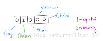
 One hot representation用来表示词向量非常简单，但是却有很多问题。最大的问题是我们的词汇表一般都非常大，比如达到百万级别，这样每个词都用百万维的向量来表示简直是内存的灾难。这样的向量其实除了一个位置是1，其余的位置全部都是0，表达的效率不高，能不能把词向量的维度变小呢？

Dristributed representation可以解决One hot representation的问题，它的思路是通过训练，将每个词都映射到一个较短的词向量上来。所有的这些词向量就构成了向量空间，进而可以用普通的统计学的方法来研究词与词之间的关系。这个较短的词向量维度是多大呢？这个一般需要我们在训练时自己来指定。

　　比如下图我们将词汇表里的词用"Royalty","Masculinity","Femininity"和"Age"4个维度来表示，King这个词对应的词向量可能是(0.99,0.99,0.05,0.7)(0.99,0.99,0.05,0.7)。当然在实际情况中，我们并不能对词向量的每个维度做一个很好的解释。

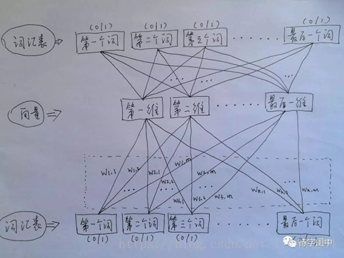
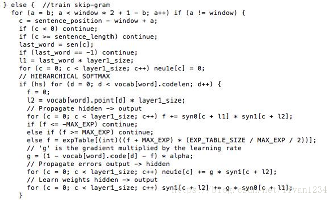
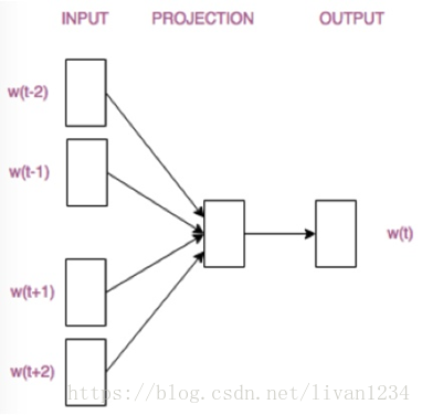
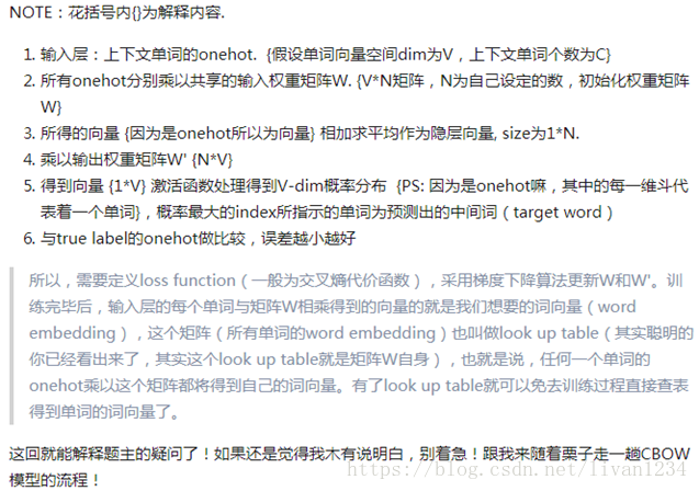
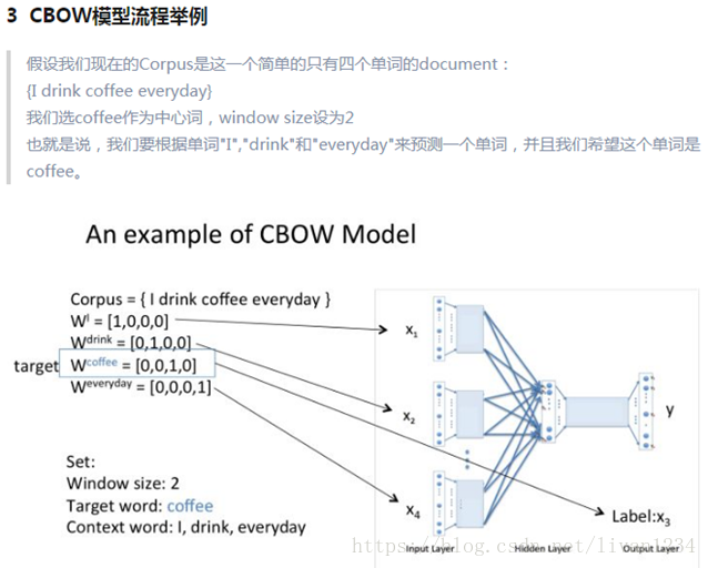
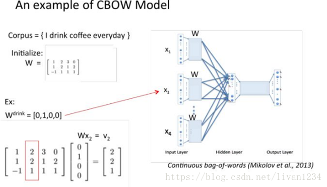
训练 Word2Vec 的思想，是利用一个词和它在文本中的上下文的词，这样就省去了人工去标注。论文中给出了 Word2Vec 的两种训练模型，CBOW (Continuous Bag-of-Words Model) 和 Skip-gram (Continuous Skip-gram Model)。

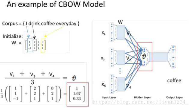
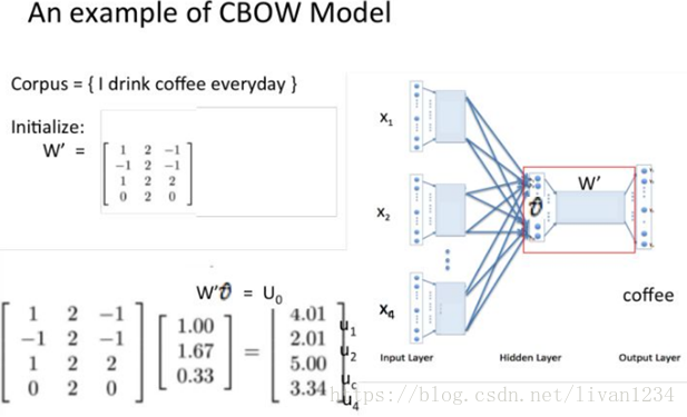
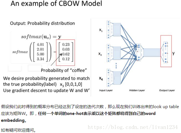
首先看CBOW，它的做法是，将一个词所在的上下文中的词作为输入，而那个词本身作为输出，也就是说，看到一个上下文，希望大概能猜出这个词和它的意思。通过在一个大的语料库训练，得到一个从输入层到隐含层的权重模型。如下图所示，第l个词的上下文词是i，j，k，那么i，j，k作为输入，它们所在的词汇表中的位置的值置为1。然后，输出是l，把它所在的词汇表中的位置的值置为1。训练完成后，就得到了每个词到隐含层的每个维度的权重，就是每个词的向量。

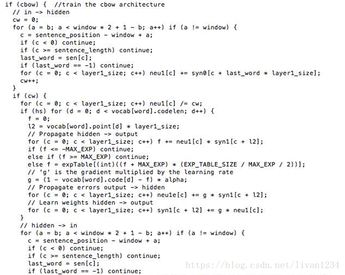
Word2Vec 代码库中关于CBOW训练的代码，其实就是神经元网路的标准反向传播算法。

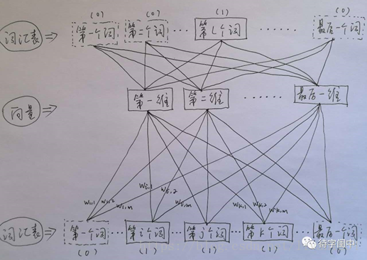
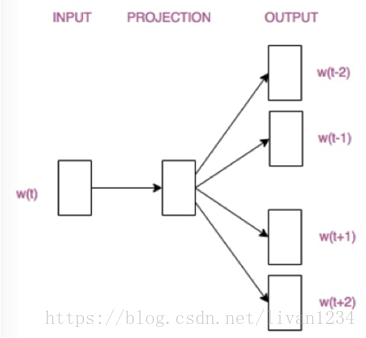
接着，看看Skip-gram，它的做法是，将一个词所在的上下文中的词作为输出，而那个词本身作为输入，也就是说，给出一个词，希望预测可能出现的上下文的词。通过在一个大的语料库训练，得到一个从输入层到隐含层的权重模型。如下图所示，第l个词的上下文词是i，j，k，那么i，j，k作为输出，它们所在的词汇表中的位置的值置为1。然后，输入是l，把它所在的词汇表中的位置的值置为1。训练完成后，就得到了每个词到隐含层的每个维度的权重，就是每个词的向量。

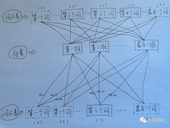
Word2Vec 代码库中关于Skip-gram训练的代码，其实就是神经元网路的标准反向传播算法。

一个人读书时，如果遇到了生僻的词，一般能根据上下文大概猜出生僻词的意思，而 Word2Vec 正是很好的捕捉了这种人类的行为，利用神经元网络模型，发现了自然语言处理的一颗原子弹。

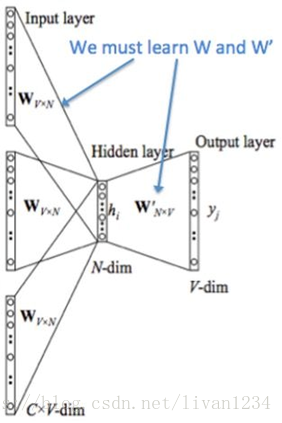
Ø  用图标来表示word2vec模型： 

CBOW模型                                    

  Skip-gram模型

 

 

 

 

二十、梯度递减优化（gradient-clip）：

tensorflow中操作gradient-clip：

在训练深度神经网络的时候,我们经常会碰到梯度消失和梯度爆炸问题,scientists提出了很多方法来解决这些问题,本篇就介绍一下如何在tensorflow中使用clip来address这些问题

train_op =tf.train.GradientDescentOptimizer(learning_rate=0.1).minimize(loss)

在调用minimize方法的时候,底层实际干了两件事:

·        计算所有 trainablevariables 梯度

·        apply them to variables

随后, 在我们 sess.run(train_op) 的时候, 会对 variables 进行更新

Clip：

那我们如果想处理一下计算完的 gradients ,那该怎么办呢? 
官方给出了以下步骤

1.    Compute the gradients withcompute_gradients(). 计算梯度

2.    Process the gradients as you wish. 处理梯度

3.    Apply the processed gradients withapply_gradients(). apply处理后的梯度给variables

这样,我们以后在train的时候就会使用 processed gradient去更新 variable 
框架:

# Create an optimizer.optimizer必须和variable在一个设备上声明

opt = GradientDescentOptimizer(learning_rate=0.1)

 

# Compute the gradients for a list of variables.

grads_and_vars = opt.compute_gradients(loss, )

 

# grads_and_vars is a list of tuples (gradient,variable).  Do whatever you

# need to the 'gradient' part, for example cap them, etc.

capped_grads_and_vars = [(MyCapper(gv[0]), gv[1]) for gv in grads_and_vars]

 

# Ask the optimizer to apply the capped gradients.

opt.apply_gradients(capped_grads_and_vars)

例子:

#return a list of trainable variable in you model

params = tf.trainable_variables()

 

#create an optimizer

opt = tf.train.GradientDescentOptimizer(self.learning_rate)

 

#compute gradients for params

gradients = tf.gradients(loss, params)

 

#process gradients

clipped_gradients, norm =tf.clip_by_global_norm(gradients,max_gradient_norm)

 

train_op = opt.apply_gradients(zip(clipped_gradients,params)))

这时, sess.run(train_op) 就可以进行训练了

 

二十一、共享变量：

为什么要共享变量？我举个简单的例子：例如，当我们研究生成对抗网络GAN的时候，判别器的任务是，如果接收到的是生成器生成的图像，判别器就尝试优化自己的网络结构来使自己输出0，如果接收到的是来自真实数据的图像，那么就尝试优化自己的网络结构来使自己输出1。也就是说，生成图像和真实图像经过判别器的时候，要共享同一套变量，所以TensorFlow引入了变量共享机制，在做卷积神经网络的时候多个卷积层有可能使用同一个权重矩阵，这时就用到了共享矩阵。

变量共享主要涉及到两个函数： tf.get_variable(, ,) 和tf.variable_scope()。

先来看第一个函数： tf.get_variable。

tf.get_variable 和tf.Variable不同的一点是，前者拥有一个变量检查机制，会检测已经存在的变量是否设置为共享变量，如果已经存在的变量没有设置为共享变量，TensorFlow 运行到第二个拥有相同名字的变量的时候，就会报错。

例如如下代码：

def my_image_filter(input_images):

    conv1_weights =tf.Variable(tf.random_normal([5, 5, 32, 32]),

       name="conv1_weights")

    conv1_biases =tf.Variable(tf.zeros([32]), name="conv1_biases")

    conv1 =tf.nn.conv2d(input_images, conv1_weights,

        strides=[1,1, 1, 1], padding='SAME')

    return  tf.nn.relu(conv1 + conv1_biases)

有两个变量(Variables)conv1_weighs, conv1_biases和一个操作(Op)conv1，如果你直接调用两次，不会出什么问题，但是会生成两套变量；

# First call creates one set of 2 variables.

result1 = my_image_filter(image1)

# Another set of 2 variables is created in the secondcall.

result2 = my_image_filter(image2)

如果把 tf.Variable 改成tf.get_variable，直接调用两次，就会出问题了：

result1 = my_image_filter(image1)

result2 = my_image_filter(image2)

# Raises ValueError(... conv1/weights already exists ...)

为了解决这个问题，TensorFlow 又提出了 tf.variable_scope函数：它的主要作用是，在一个作用域 scope 内共享一些变量，可以有如下几种用法：

1）

with tf.variable_scope("image_filters") asscope:

    result1 =my_image_filter(image1)

   scope.reuse_variables() # or

   #tf.get_variable_scope().reuse_variables()

    result2 =my_image_filter(image2)

需要注意的是：最好不要设置 reuse 标识为False，只在需要的时候设置 reuse 标识为True。

2)

with tf.variable_scope("image_filters1") asscope1:

    result1 =my_image_filter(image1)

with tf.variable_scope(scope1, reuse = True)

    result2 =my_image_filter(image2)

通常情况下，tf.variable_scope 和tf.name_scope 配合，能画出非常漂亮的流程图，但是他们两个之间又有着细微的差别，那就是 name_scope 只能管住操作 Ops的名字，而管不住变量 Variables 的名字，看下例：

with tf.variable_scope("foo"):

    withtf.name_scope("bar"):

        v = tf.get_variable("v", [1])

        x = 1.0 + v

assert v.name == "foo/v:0"

assert x.op.name == "foo/bar/add"

 

在tensorflow中,有两个scope, 一个是name_scope一个是variable_scope,这两个scope到底有什么区别呢? 
先看第一个程序:

with tf.name_scope("hello") as name_scope:

    arr1 = tf.get_variable("arr1", shape=[2,10],dtype=tf.float32)

# 输出

var1/w:0

name1/var1/Add:0

可以看出：

·        variable scope和name scope都会给op的name加上前缀 

·        这实际上是因为创建 variable_scope 时内部会创建一个同名的 name_scope

对比三个个程序可以看出:

·        name_scope 返回的是 string, 而 variable_scope 返回的是对象. 这也可以感觉到, variable_scope 能干的事情比 name_scope 要多.

·        name_scope对 get_variable()创建的变量的名字不会有任何影响,而创建的op会被加上前缀.

·        tf.get_variable_scope() 返回的只是 variable_scope,不管 name_scope. 所以以后我们在使用tf.get_variable_scope().reuse_variables()时可以无视name_scope

其它

with tf.name_scope("scope1") as scope1:

    with tf.name_scope("scope2") as scope2:

        print scope2

#输出：scope1/scope2/

import tensorflow as tf

with tf.variable_scope("scope1") as scope1:

    with tf.variable_scope("scope2") as scope2:

        print scope2.name

#输出:scope1/scope2

name_scope可以用来干什么

典型的 TensorFlow 可以有数以千计的节点，如此多而难以一下全部看到，甚至无法使用标准图表工具来展示。为简单起见，我们为op/tensor名划定范围，并且可视化把该信息用于在图表中的节点上定义一个层级。默认情况下， 只有顶层节点会显示。下面这个例子使用tf.name_scope在hidden命名域下定义了三个操作:

import tensorflow as tf

with tf.name_scope('hidden') as scope:

  a = tf.constant(5, name='alpha')

  W = tf.Variable(tf.random_uniform([1, 2], -1.0, 1.0), name='weights')

  b = tf.Variable(tf.zeros([1]), name='biases')

  print a.name

  print W.name

  print b.name

结果是得到了下面三个操作名:

hidden/alpha 
hidden/weights 
hidden/biases 
name_scope 是给op_name加前缀,variable_scope是给get_variable()创建的变量的名字加前缀。

tf.variable_scope有时也会处理命名冲突

import tensorflow as tf

def test(name=None):

    with tf.variable_scope(name, default_name="scope") as scope:

        w = tf.get_variable("w", shape=[2, 10])

#scope/w:0

#scope_1/w:0

#可以看出，如果只是使用default_name这个属性来创建variable_scope

#的时候，会处理命名冲突

其它

·        tf.name_scope(None) 有清除name scope的作用

import tensorflow as tf

with tf.name_scope("hehe"):

    w1 = tf.Variable(1.0)

    with tf.name_scope(None):

        w2 = tf.Variable(2.0)

#hehe/Variable:0

#Variable:0

总结

简单来看 
1. 使用tf.Variable()的时候，tf.name_scope()和tf.variable_scope() 都会给 Variable 和 op 的 name属性加上前缀。 
2. 使用tf.get_variable()的时候，tf.name_scope()就不会给 tf.get_variable()创建出来的Variable加前缀。但是 tf.Variable() 创建出来的就会受到 name_scope 的影响.

 

二十二、run_cell常用方法：

主要是神经网络cell中的内容：

Ø  run_cell._linear()

def_linear(args,output_size, bias, bias_start=0.0, scope=None):

·        args: list of tensor [batch_size, size]. 注意,list中的每个tensor的size 并不需要一定相同,但batch_size要保证一样.

·        output_size : 一个整数

·        bias: bool型, True表示加bias,False表示不加

·        return : [batch_size, output_size] 
注意: 这个函数的atgs 不能是 _ref 类型(tf_getvariable(), tf.Variables()返回的都是 _ref),但这个 _ref类型经过任何op之后,_ref就会消失

PS: _ref referente-typed is mutable

Ø  rnn_cell.BasicLSTMCell()

classBasicLSTMCell(RNNCell):

  def__init__(self,num_units, forget_bias=1.0,input_size=None,

              state_is_tuple=True, activation=tanh):

"""

为什么被称为 Basic

It does not allow cell clipping, a projection layer, anddoes not

use peep-hole connections: it is the basic baseline.

"""

·        num_units: lstm单元的output_size

·        input_size: 这个参数没必要输入, 官方说马上也要禁用了

·        state_is_tuple: True的话, (c_state,h_state)作为tuple返回

·        activation: 激活函数 
注意: 在我们创建 cell=BasicLSTMCell(…) 的时候, 只是初始化了cell的一些基本参数值. 这时,是没有variable被创建的, variable在我们 cell(input, state)时才会被创建, 下面所有的类都是这样

rnn_cell.GRUCell()

classGRUCell(RNNCell):

  def__init__(self,num_units, input_size=None, activation=tanh):

创建一个GRUCell

rnn_cell.LSTMCell()

classLSTMCell(RNNCell):

  def__init__(self,num_units, input_size=None,

              use_peepholes=False, cell_clip=None,

              initializer=None, num_proj=None, proj_clip=None,

              num_unit_shards=1, num_proj_shards=1,

              forget_bias=1.0, state_is_tuple=True,

              activation=tanh):          

·        num_proj: python Innteger ,映射输出的size, 用了这个就不需要下面那个类了

rnn_cell.OutputProjectionWrapper()

classOutputProjectionWrapper(RNNCell):

  def__init__(self,cell, output_size):

·        output_size: 要映射的 size

·        return: 返回一个带有 OutputProjection Layer的 cell(s)

rnn_cell.InputProjectionWrapper():

classInputProjectionWrapper(RNNCell):

  def__init__(self,cell, num_proj, input_size=None):

·        和上面差不多,一个输出映射,一个输入映射

rnn_cell.DropoutWrapper()

classDropoutWrapper(RNNCell):

  def__init__(self,cell, input_keep_prob=1.0,output_keep_prob=1.0,

              seed=None):

·        dropout

rnn_cell.EmbeddingWrapper():

classEmbeddingWrapper(RNNCell):

  def__init__(self,cell, embedding_classes, embedding_size, initializer=None):

·        返回一个带有 embedding 的cell

rnn_cell.MultiRNNCell():

classMultiRNNCell(RNNCell):

  def__init__(self,cells, state_is_tuple=True):

·        用来增加 rnn 的层数

·        cells : list of cell

·        返回一个多层的 cell

二十三、tensorboard可视化：

tensorflow的可视化是使用summary和tensorboard合作完成的.

基本用法

首先明确一点,summary也是op.

输出网络结构

with tf.Session() as sess:

  writer =tf.summary.FileWriter(your_dir, sess.graph)

命令行运行tensorboard--logdir your_dir,然后浏览器输入127.0.1.1:6006注：tf1.1.0 版本的tensorboard端口换了(0.0.0.0:6006) 
这样你就可以在tensorboard中看到你的网络结构图了

可视化参数

#ops

loss = ...

tf.summary.scalar("loss", loss)

merged_summary = tf.summary.merge_all()

init = tf.global_variable_initializer()

with tf.Session() as sess:

    writer= tf.summary.FileWriter(your_dir, sess.graph)

    sess.run(init)

    for i in xrange(100):

        _,summary =sess.run([train_op,merged_summary], feed_dict)

        writer.add_summary(summary, i)

这时,打开tensorboard,在EVENTS可以看到loss随着i的变化了，如果看不到的话，可以在代码最后加上writer.flush()试一下，原因后面说明。

函数介绍

·        tf.summary.merge_all: 将之前定义的所有summary op整合到一起

·        FileWriter: 创建一个filewriter用来向硬盘写summary数据,

·        tf.summary.scalar(summary_tags,Tensor/variable, collections=None): 用于标量的 summary

·        tf.summary.image(tag, tensor, max_images=3,collections=None, name=None):tensor,必须4维,形状[batch_size, height, width, channels],max_images(最多只能生成3张图片的summary),觉着这个用在卷积中的kernel可视化很好用.max_images确定了生成的图片是[-max_images: ,height, width, channels]，还有一点就是，TensorBord中看到的imagesummary永远是最后一个global step的

·        tf.summary.histogram(tag, values,collections=None, name=None):values,任意形状的tensor,生成直方图summary

·        tf.summary.audio(tag, tensor, sample_rate,max_outputs=3, collections=None, name=None)

解释collections参数：它是一个list,如果不指定collections, 那么此summary会被添加到f.GraphKeys.SUMMARIES中，如果指定了，就会放在的collections中。

FileWriter

注意:add_summary仅仅是向FileWriter对象的缓存中存放event data。而向disk上写数据是由FileWrite对象控制的。下面通过FileWriter的构造函数来介绍这一点！！！

tf.summary.FileWriter.__init__(logdir, graph=None, max_queue=10,flush_secs=120, graph_def=None)

Creates a FileWriter and an eventfile.

# max_queue: 在向disk写数据之前，最大能够缓存event的个数

# flush_secs: 每多少秒像disk中写数据，并清空对象缓存

注意

1.    如果使用writer.add_summary(summary，global_step)时没有传global_step参数,会使scarlar_summary变成一条直线。

2.    只要是在计算图上的Summary op，都会被merge_all捕捉到， 不需要考虑变量生命周期问题！

3.    如果执行一次，disk上没有保存Summary数据的话，可以尝试下file_writer.flush()

小技巧

如果想要生成的summary有层次的话，记得在summary外面加一个name_scope

with tf.name_scope("summary_gradients"):

   tf.summary.histgram("name", gradients)

这样，tensorboard在显示的时候，就会有一个sumary_gradients一级目录。

最近在研究tensorflow自带的例程speech_command,顺便学习tensorflow的一些基本用法。

其中tensorboard 作为一款可视化神器，可以说是学习tensorflow时模型训练以及参数可视化的法宝。

而在训练过程中，主要用到了tf.summary()的各类方法，能够保存训练过程以及参数分布图并在tensorboard显示。

tf.summary有诸多函数：

1、tf.summary.scalar

用来显示标量信息，其格式为：

tf.summary.scalar(tags, values, collections=None,name=None)

例如：tf.summary.scalar('mean', mean)

一般在画loss,accuary时会用到这个函数。

2、tf.summary.histogram

用来显示直方图信息，其格式为：

tf.summary.histogram(tags, values, collections=None,name=None)

例如： tf.summary.histogram('histogram',var)

一般用来显示训练过程中变量的分布情况

3、tf.summary.distribution

分布图，一般用于显示weights分布

4、tf.summary.text

可以将文本类型的数据转换为tensor写入summary中：

例如：

text ="""/a/b/c\\_d/f\\_g\\_h\\_2017"""

summary_op0 = tf.summary.text('text',tf.convert_to_tensor(text))

5、tf.summary.image

输出带图像的probuf，汇总数据的图像的的形式如下： ' tag /image/0',' tag /image/1'...，如：input/image/0等。

格式：tf.summary.image(tag, tensor, max_images=3, collections=None, name=Non

6、tf.summary.audio

展示训练过程中记录的音频 

7、tf.summary.merge_all

merge_all 可以将所有summary全部保存到磁盘，以便tensorboard显示。如果没有特殊要求，一般用这一句就可一显示训练时的各种信息了。

格式：tf.summaries.merge_all(key='summaries')

8、tf.summary.FileWriter

指定一个文件用来保存图。

格式：tf.summary.FileWritter(path,sess.graph)

可以调用其add_summary（）方法将训练过程数据保存在filewriter指定的文件中

Tensorflow Summary 用法示例:

tf.summary.scalar('accuracy',acc)                   #生成准确率标量图 

merge_summary = tf.summary.merge_all() 

train_writer = tf.summary.FileWriter(dir,sess.graph)#定义一个写入summary的目标文件，dir为写入文件地址 

......(交叉熵、优化器等定义) 

for step in xrange(training_step):                  #训练循环 

    train_summary =sess.run(merge_summary,feed_dict = {...})#调用sess.run运行图，生成一步的训练过程数据 

    train_writer.add_summary(train_summary,step)#调用train_writer的add_summary方法将训练过程以及训练步数保存 

此时开启tensorborad：

tensorboard --logdir=/summary_dir 

便能看见accuracy曲线了。

另外，如果我不想保存所有定义的summary信息，也可以用tf.summary.merge方法有选择性地保存信息：

9、tf.summary.merge

格式：tf.summary.merge(inputs, collections=None,name=None)

一般选择要保存的信息还需要用到tf.get_collection()函数

示例：

tf.summary.scalar('accuracy',acc)                   #生成准确率标量图 

merge_summary =tf.summary.merge([tf.get_collection(tf.GraphKeys.SUMMARIES,'accuracy'),...(其他要显示的信息)]) 

train_writer = tf.summary.FileWriter(dir,sess.graph)#定义一个写入summary的目标文件，dir为写入文件地址 

......(交叉熵、优化器等定义) 

for step in xrange(training_step):                  #训练循环 

    train_summary =sess.run(merge_summary,feed_dict = {...})#调用sess.run运行图，生成一步的训练过程数据 

    train_writer.add_summary(train_summary,step)#调用train_writer的add_summary方法将训练过程以及训练步数保存 

使用tf.get_collection函数筛选图中summary信息中的accuracy信息，这里的

tf.GraphKeys.SUMMARIES  是summary在collection中的标志。

当然，也可以直接：

acc_summary = tf.summary.scalar('accuracy',acc)                   #生成准确率标量图 

merge_summary = tf.summary.merge([acc_summary ,...(其他要显示的信息)])  #这里的[]不可省

二十四、tensorflow configProto

tf.ConfigProto一般用在创建session的时候。用来对session进行参数配置

with tf.Session(config = tf.ConfigProto(...),...)

#tf.ConfigProto()的参数

log_device_placement=True : 是否打印设备分配日志

allow_soft_placement=True：如果你指定的设备不存在，允许TF自动分配设备

tf.ConfigProto(log_device_placement=True,allow_soft_placement=True)

Ø  控制GPU资源使用率

#allow growth

config = tf.ConfigProto()

config.gpu_options.allow_growth = True

session = tf.Session(config=config, ...)

# 使用allow_growthoption，刚一开始分配少量的GPU容量，然后按需慢慢的增加，由于不会释放

#内存，所以会导致碎片

# per_process_gpu_memory_fraction

gpu_options=tf.GPUOptions(per_process_gpu_memory_fraction=0.7)

config=tf.ConfigProto(gpu_options=gpu_options)

session = tf.Session(config=config, ...)

#设置每个GPU应该拿出多少容量给进程使用，0.4代表 40%

Ø  控制使用哪块GPU

~/ CUDA_VISIBLE_DEVICES=0  python your.py#使用GPU0

~/ CUDA_VISIBLE_DEVICES=0,1 pythonyour.py#使用GPU0,1

#注意单词不要打错

 

#或者在程序开头

os.environ['CUDA_VISIBLE_DEVICES'] = '0'#使用 GPU 0

os.environ['CUDA_VISIBLE_DEVICES'] = '0,1'# 使用 GPU 0，1

二十五、如何构建TF代码

batch_size: batch的大小 
mini_batch: 将训练样本以batch_size分组 
epoch_size: 样本分为几个min_batch 
num_epoch : 训练几轮

读代码的时候应该关注的几部分

1.    如何处理数据

2.    如何构建计算图

3.    如何计算梯度

4.    如何Summary，如何save模型参数

5.    如何执行计算图

写一个将数据分成训练集,验证集和测试集的函数

train_set, valid_set, test_set = split_set(data)

最好写一个管理数据的对象，将原始数据转化成mini_batch

classDataManager(object):

  #raw_data为train_set, valid_data或test_set

  def__init__(self,raw_data, batch_size):

    self.raw_data =raw_data

    self.batch_size= batch_size

    self.epoch_size= len(raw_data)/batch_size

    self.counter = 0#监测batch index

  defnext_batch(self):

    ...

    self.counter +=1

    return batched_x,batched_label, ...

计算图的构建在Model类中的__init__()中完成,并设置is_training参数

优点： 
1. 因为如果我们在训练的时候加dropout的话，那么在测试的时候是需要把这个dropout层去掉的。这样的话，在写代码的时候，你就可以创建两个对象。这就相当于建了两个模型，然后让这两个模型参数共享，就可以达到训练和测试一起运行的效果了。具体看下面代码。

classModel(object):

  def__init__(self,is_training, config, scope,...):#scope可以使你正确的summary

   self.is_training = is_training

    self.config =config

    #placeholder:用于feed数据

    # 一个train op

   self.graph(self.is_training) #构建图

    self.merge_op =tf.summary.merge(tf.get_collection(tf.GraphKeys.SUMMARIES,scope))

  defgraph(self,is_training):

    ...

    #定义计算图

    self.predict =...

    self.loss = ...

写个run_epoch函数

batch_size: batch的大小 
mini_batch: 将训练样本以batch_size分组 
epoch_size: 样本分为几个min_batch 
num_epoch : 训练几轮 
如何编写run_epoch函数

#eval_op是用来指定是否需要训练模型，需要的话，传入模型的eval_op

#draw_ata用于接收train_data,valid_data或test_data

defrun_epoch(raw_data ，session, model, is_training_set, ...):

  data_manager =DataManager(raw_data, model.config.batch_size)

 

  #通过is_training_set来决定fetch哪些Tensor

  #add_summary,saver.save(....)

如何组织main函数

1.    分解原始数据为train，valid，test

2.    设置默认图

3.    建图 trian, test 分别建图

4.    一个或多个Saver对象，用来保存模型参数

5.    创建session，初始化变量

6.    一个summary.FileWriter对象，用来将summary写入到硬盘中

7.    run epoch

FileWriter 和 Saver对象，一个计算图只需要一个就够了，所以放在Model类的外面

附录

本篇博文总结下面代码写成， 有些地方和源码之间有不同。 
下面是截取自官方代码：

classPTBInput(object):

  """Theinput data."""

 

  def__init__(self,config, data, name=None):

    self.batch_size= batch_size = config.batch_size

    self.num_steps= num_steps = config.num_steps

    self.epoch_size= ((len(data) // batch_size) - 1) // num_steps

   self.input_data, self.targets = reader.ptb_producer(

        data,batch_size, num_steps, name=name)

classPTBModel(object):

  """ThePTB model."""

 

  def__init__(self,is_training, config, input_):

    self._input =input_

 

    batch_size =input_.batch_size

    num_steps =input_.num_steps

    size =config.hidden_size

    vocab_size =config.vocab_size

 

    # Slightlybetter results can be obtained with forget gate biases

    #initialized to 1 but the hyperparameters of the model would need to be

    # different than reported in thepaper.

    lstm_cell =tf.contrib.rnn.BasicLSTMCell(

        size,forget_bias=0.0, state_is_tuple=True)

    if is_trainingand config.keep_prob < 1:

      lstm_cell =tf.contrib.rnn.DropoutWrapper(

         lstm_cell, output_keep_prob=config.keep_prob)

    cell =tf.contrib.rnn.MultiRNNCell(

        [lstm_cell]* config.num_layers, state_is_tuple=True)

 

   self._initial_state = cell.zero_state(batch_size, data_type())

 

    with tf.device("/cpu:0"):

      embedding =tf.get_variable(

          "embedding",[vocab_size, size], dtype=data_type())

      inputs =tf.nn.embedding_lookup(embedding, input_.input_data)

 

    if is_trainingand config.keep_prob < 1:

      inputs =tf.nn.dropout(inputs, config.keep_prob)

 

    #Simplified version of models/tutorials/rnn/rnn.py's rnn().

    # Thisbuilds an unrolled LSTM for tutorial purposes only.

    # Ingeneral, use the rnn() or state_saving_rnn() from rnn.py.

    #

    # Thealternative version of the code below is:

    #

    # inputs =tf.unstack(inputs, num=num_steps, axis=1)

    # outputs,state = tf.nn.rnn(cell, inputs,

    #                           initial_state=self._initial_state)

    outputs = []

    state =self._initial_state

    withtf.variable_scope("RNN"):

      for time_step inrange(num_steps):

        if time_step> 0: tf.get_variable_scope().reuse_variables()

       (cell_output, state) = cell(inputs[:, time_step, :], state)

       outputs.append(cell_output)

 

    output =tf.reshape(tf.concat_v2(outputs, 1), [-1, size])

    softmax_w =tf.get_variable(

        "softmax_w", [size,vocab_size], dtype=data_type())

    softmax_b =tf.get_variable("softmax_b", [vocab_size],dtype=data_type())

    logits =tf.matmul(output, softmax_w) + softmax_b

    loss =tf.contrib.legacy_seq2seq.sequence_loss_by_example(

        [logits],

       [tf.reshape(input_.targets, [-1])],

       [tf.ones([batch_size * num_steps], dtype=data_type())])

    self._cost =cost = tf.reduce_sum(loss) / batch_size

   self._final_state = state

 

    ifnotis_training:

      return

 

    self._lr =tf.Variable(0.0, trainable=False)

    tvars =tf.trainable_variables()

    grads, _ =tf.clip_by_global_norm(tf.gradients(cost, tvars),

                                     config.max_grad_norm)

    optimizer =tf.train.GradientDescentOptimizer(self._lr)

    self._train_op= optimizer.apply_gradients(

        zip(grads,tvars),

       global_step=tf.contrib.framework.get_or_create_global_step())

 

    self._new_lr =tf.placeholder(

        tf.float32,shape=[], name="new_learning_rate")

    self._lr_update= tf.assign(self._lr, self._new_lr)

 

  defassign_lr(self,session, lr_value):

   session.run(self._lr_update, feed_dict={self._new_lr: lr_value})

 

defrun_epoch(session,model, eval_op=None, verbose=False):

  """Runsthe model on the given data."""

  start_time =time.time()

  costs = 0.0

  iters = 0

  state =session.run(model.initial_state)

 

  fetches = {

      "cost":model.cost,

      "final_state":model.final_state,

  }

  if eval_op isnotNone:

    fetches["eval_op"] = eval_op

 

  for step inrange(model.input.epoch_size):

    feed_dict = {}

    for i, (c, h) inenumerate(model.initial_state):

      feed_dict[c]= state[i].c

      feed_dict[h]= state[i].h

 

    vals =session.run(fetches, feed_dict)

    cost = vals["cost"]

    state = vals["final_state"]

 

    costs += cost

    iters +=model.input.num_steps

 

    if verbose and step %(model.input.epoch_size // 10) == 10:

      print("%.3fperplexity: %.3f speed: %.0f wps" %

            (step *1.0 / model.input.epoch_size, np.exp(costs /iters),

             iters* model.input.batch_size / (time.time() - start_time)))

 

  returnnp.exp(costs / iters)

 

defmain(_):

  ifnotFLAGS.data_path:

    raise ValueError("Mustset --data_path to PTB data directory")

 

  raw_data =reader.ptb_raw_data(FLAGS.data_path)

  train_data,valid_data, test_data, _ = raw_data

 

  config =get_config()

  eval_config =get_config()

 eval_config.batch_size = 1

 eval_config.num_steps = 1

 

  withtf.Graph().as_default():

    initializer =tf.random_uniform_initializer(-config.init_scale,

                                                config.init_scale)

 

    withtf.name_scope("Train"):

      train_input =PTBInput(config=config, data=train_data, name="TrainInput")

      withtf.variable_scope("Model", reuse=None,initializer=initializer):

        m =PTBModel(is_training=True, config=config,input_=train_input)

     tf.contrib.deprecated.scalar_summary("TrainingLoss", m.cost)

     tf.contrib.deprecated.scalar_summary("LearningRate", m.lr)

 

    withtf.name_scope("Valid"):

      valid_input =PTBInput(config=config, data=valid_data, name="ValidInput")

      withtf.variable_scope("Model", reuse=True,initializer=initializer):

        mvalid =PTBModel(is_training=False,config=config, input_=valid_input)

     tf.contrib.deprecated.scalar_summary("ValidationLoss", mvalid.cost)

 

    withtf.name_scope("Test"):

      test_input =PTBInput(config=eval_config, data=test_data, name="TestInput")

      withtf.variable_scope("Model", reuse=True,initializer=initializer):

        mtest =PTBModel(is_training=False,config=eval_config,

                        input_=test_input)

 

    sv =tf.train.Supervisor(logdir=FLAGS.save_path)

    withsv.managed_session() as session:

      for i inrange(config.max_max_epoch):

        lr_decay =config.lr_decay ** max(i + 1 - config.max_epoch, 0.0)

       m.assign_lr(session, config.learning_rate * lr_decay)

 

        print("Epoch:%d Learning rate: %.3f" % (i + 1,session.run(m.lr)))

       train_perplexity = run_epoch(session, m, eval_op=m.train_op,

                                     verbose=True)

        print("Epoch:%d Train Perplexity: %.3f" % (i + 1,train_perplexity))

       valid_perplexity = run_epoch(session, mvalid)

        print("Epoch:%d Valid Perplexity: %.3f" % (i + 1,valid_perplexity))

 

     test_perplexity = run_epoch(session, mtest)

      print("TestPerplexity: %.3f" % test_perplexity)

 

      ifFLAGS.save_path:

        print("Savingmodel to %s." % FLAGS.save_path)

       sv.saver.save(session, FLAGS.save_path, global_step=sv.global_step)

 

 

if __name__ == "__main__":

  tf.app.run()

二十六、collection全局存储

tensorflow的collection提供一个全局的存储机制，不会受到变量名生存空间的影响。一处保存，到处可取。

接口介绍

#向collection中存数据

tf.Graph.add_to_collection(name, value)

 

#Stores value in the collection with the given name.

#Note that collections are not sets, so it is possible toadd a value to a collection

#several times.

# 注意，一个‘name’下，可以存很多值; add_to_collection("haha",[a,b]),这种情况下

#tf.get_collection("haha")获得的是 [[a,b]], 并不是[a,b]

tf.add_to_collection(name, value)

#这个和上面函数功能上没有区别，区别是，这个函数是给默认图使用的

#从collection中获取数据

tf.Graph.get_collection(name, scope=None)

二十七、merge_all的应用

不要用merge_all而是用merge。

1.   在训练深度神经网络的时候，我们经常会使用Dropout，然而在test的时候，需要把dropout撤掉.为了应对这种问题，我们通常要建立两个模型，让他们共享变量。详情.也可以通过设置 train_flag, 这里只讨论第一个方法可能会碰到的问题.

2.   为了使用Tensorboard来可视化我们的数据，我们会经常使用Summary，最终都会用一个简单的merge_all函数来管理我们的Summary

错误示例

当这两种情况相遇时，bug就产生了，看代码：

import tensorflow as tf

import numpy as np

class Model(object):

    def __init__(self):

def run_epoch(session, model):

    x = np.random.rand(1000).reshape(-1,1)

    label = x*3

def main():

    with tf.Graph().as_default():

        with tf.name_scope("train"):

            with tf.variable_scope("var1",dtype=tf.float32):

class Model(object):

    def __init__(self):

class Model(object):

    def __init__(self，scope):

def multi_gpu_model(num_gpus=1):

def generate_feed_dic(model, feed_dict, batch_generator):

#这里的scope是用来区别 train 还是 test

def run_epoch(session, data_set, scope, train_op=None, is_training=True):

# 建图完毕，开始执行运算

with tf.Session() as sess:

def average_gradients(grads):#grads:[[grad0, grad1,..], [grad0,grad1,..]..]

def average_gradients(grads):#grads:[[grad0, grad1,..], [grad0,grad1,..]..]

# 以 w 当作 key， 获取 shadow value 的值

ema_val = ema.average(w)#参数不能是list，有点蛋疼

with tf.Session() as sess:

# 创建一个时间序列 1 2 3 4

#输出：

#1.1      =0.9*1 + 0.1*2

#1.29     =0.9*1.1+0.1*3

#1.561    =0.9*1.29+0.1*4

你可能会奇怪，明明 只执行三次循环， 为什么产生了 4 个数？ 
这是因为，当程序执行到 ema_op = ema.apply([w]) 的时候，如果 w 是 Variable， 那么将会用 w 的初始值初始化 ema 中关于 w 的 ema_value，所以 emaVal0=1.0emaVal0=1.0。如果 w 是 Tensor的话，将会用 0.0 初始化。

官网中的示例：

# Create variables.

# ... use the variables to build a training model...

# Create an op that applies the optimizer.  This is what we usually

# would use as a training op.

# Create an ExponentialMovingAverage object

ema = tf.train.ExponentialMovingAverage(decay=0.9999)

# Create the shadow variables, and add ops to maintain moving averages

# of var0 and var1.

# Create an op that will update the moving averages after each training

# step.  This is what we will use in place of the usual training op.

with tf.control_dependencies([opt_op]):

# Create a Saver that loads variables from their saved shadow values.

# var0 and var1 now hold the moving average values

方法二：

#Returns a map of names to Variables to restore.

# Pass the variables as a dict:

saver = tf.train.Saver({'v1': v1, 'v2': v2})

# Or pass them as a list.

# Passing a list is equivalent to passing a dict with the variable op names

# as keys:

saver = tf.train.Saver({v.op.name: v for v in [v1, v2]})

#注意，如果不给Saver传var_list 参数的话， 他将已 所有可以保存的 variable作为其var_list的值。

这里使用了三种不同的方式来创建 saver 对象， 但是它们内部的原理是一样的。我们都知道，参数会保存到 checkpoint 文件中，通过键值对的形式在 checkpoint中存放着。如果 Saver 的构造函数中传的是 dict，那么在 save 的时候，checkpoint文件中存放的就是对应的 key-value。如下：

import tensorflow as tf

# Create some variables.

v1 = tf.Variable(1.0, name="v1")

v2 = tf.Variable(2.0, name="v2")

saver = tf.train.Saver({"variable_1":v1, "variable_2": v2})

# Use the saver object normally after that.

with tf.Session() as sess:

# 输出:

#tensor_name:  variable_1

#1.0

#tensor_name:  variable_2

#2.0

如果构建saver对象的时候，我们传入的是 list， 那么将会用对应 Variable 的 variable.op.name 作为 key。

import tensorflow as tf

# Create some variables.

v1 = tf.Variable(1.0, name="v1")

v2 = tf.Variable(2.0, name="v2")

# Use the saver object normally after that.

with tf.Session() as sess:

1.0

2.0

如果我们现在想将 checkpoint 中v2的值restore到v1 中，v1的值restore到v2中，我们该怎么做？ 
这时，我们只能采用基于 dict 的 saver

import tensorflow as tf

# Create some variables.

v1 = tf.Variable(1.0, name="v1")

v2 = tf.Variable(2.0, name="v2")

saver = tf.train.Saver({"variable_1":v1, "variable_2": v2})

# Use the saver object normally after that.

with tf.Session() as sess:

# Create some variables.

v1 = tf.Variable(1.0, name="v1")

v2 = tf.Variable(2.0, name="v2")

#restore的时候，variable_1对应到v2，variable_2对应到v1，就可以实现目的了。

saver = tf.train.Saver({"variable_1":v2, "variable_2": v1})

# Use the saver object normally after that.

with tf.Session() as sess:

# 输出的结果是 2.0 1.0，如我们所望

我们发现，其实 创建 saver对象时使用的键值对就是表达了一种对应关系：

·        save时，表示：variable的值应该保存到 checkpoint文件中的哪个 key下

·        restore时，表示：checkpoint文件中key对应的值，应该restore到哪个variable

其它

一个快速找到ckpt文件的方式

# sess.run(group)和sess.run(tuple)都会求Tensor(add)

#Tensor(mul)的值。区别是，tf.group()返回的是`op`

#tf.tuple()返回的是list of tensor。

#这样就会导致，sess.run(tuple)的时候，会返回 Tensor(mul),Tensor(add)的值.

#而 sess.run(group)不会

tf.identity()

http://stackoverflow.com/questions/34877523/in-tensorflow-what-is-tf-identity-used-for

tf.while_loop()

tf.while_loop(cond, body, loop_vars,shape_invariants=None, parallel_iterations=10, back_prop=True,swap_memory=False, name=None)

while_loop可以这么理解

# Definition of condition and body

def cond(a, b, f):

    return a < 3

def body(a, b, f):

    # do some stuff with a, b

    a = a + 1

    return a, b, f

# Loop, 返回的tensor while 循环后的 a，b，f；[a,b,f]是返回值。

# ....

多层双向rnn

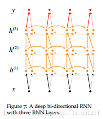
多层双向rnn(cs224d)

单层双向rnn可以通过上述方法简单的实现,但是多层的双向rnn就不能使将MultiRNNCell传给bidirectional_dynamic_rnn了. 
想要知道为什么,我们需要看一下bidirectional_dynamic_rnn的源码片段.

with vs.variable_scope(scope or "bidirectional_rnn"):

  # Forward direction

  with vs.variable_scope("fw") as fw_scope:

def _reverse(input_, seq_lengths, seq_dim, batch_dim):

  if seq_lengths is not None:

    return array_ops.reverse_sequence(

# Given this:

batch_dim = 0

seq_dim = 1

input.dims = (4, 8, ...)

seq_lengths = [7, 2, 3, 5]

# then slices of input are reversed on seq_dim, but only up to seq_lengths:

output[0, 0:7, :, ...] = input[0, 7:0:-1, :, ...]

output[1, 0:2, :, ...] = input[1, 2:0:-1, :, ...]

output[2, 0:3, :, ...] = input[2, 3:0:-1, :, ...]

output[3, 0:5, :, ...] = input[3, 5:0:-1, :, ...]

# while entries past seq_lens are copied through:

output[0, 7:, :, ...] = input[0, 7:, :, ...]

output[1, 2:, :, ...] = input[1, 2:, :, ...]

output[2, 3:, :, ...] = input[2, 3:, :, ...]

output[3, 2:, :, ...] = input[3, 2:, :, ...]

例二:

# Given this:

batch_dim = 2

seq_dim = 0

input.dims = (8, ?, 4, ...)

seq_lengths = [7, 2, 3, 5]

# then slices of input are reversed on seq_dim, but only up to seq_lengths:

output[0:7, :, 0, :, ...] = input[7:0:-1, :, 0, :, ...]

output[0:2, :, 1, :, ...] = input[2:0:-1, :, 1, :, ...]

output[0:3, :, 2, :, ...] = input[3:0:-1, :, 2, :, ...]

output[0:5, :, 3, :, ...] = input[5:0:-1, :, 3, :, ...]

# while entries past seq_lens are copied through:

output[7:, :, 0, :, ...] = input[7:, :, 0, :, ...]

output[2:, :, 1, :, ...] = input[2:, :, 1, :, ...]

output[3:, :, 2, :, ...] = input[3:, :, 2, :, ...]

output[2:, :, 3, :, ...] = input[2:, :, 3, :, ...]

三十八、control dependencies

tf.control_dependencies()设计是用来控制计算流图的，给图中的某些计算指定顺序。比如：我们想要获取参数更新后的值，那么我们可以这么组织我们的代码。

#这段代码出现在Variable类定义文件中第287行，

# 在创建Varible时，tensorflow是移除了dependencies了的

#所以会出现 control 不住的情况

with ops.control_dependencies(None):

# 第一行： 引包

from tensorflow.python import debug as tf_debug

# 初始化的 sess 没必要加上 debug wrapper

# 第二行，给 session 加个 wrapper

# 或者

# enqueue_many 的写法，两个元素放在两个列表里。

en_m = queue.enqueue_many([['hello', 'world'], [1, 2]])

# enqueue 的写法

en = queue.enqueue(['hello', 1])

deq = queue.dequeue()

with tf.Session() as sess:

    sess.run(en_m)

    print(sess.run(deq))

四十二、session.run()的解释

当我们训练自己的神经网络的时候，无一例外的就是都会加上一句 sess.run(tf.global_variables_initializer()) ，这行代码的官方解释是 初始化模型的参数。那么，它到底做了些什么？

在执行tensor的时候，你可以使用sess.run()在同一步获取多个tensor中的值，使用Tensor.eval()时只能在同一步当中获取一个tensor值，并且每次使用 eval 和 run时，都会执行整个计算图。

一步步看源代码：（代码在后面）

·        global_variables_initializer 返回一个用来初始化计算图中所有globalvariable的 op。 
 

·        这个op 到底是啥，还不清楚。

·        函数中调用了 variable_initializer() 和 global_variables()

·        global_variables() 返回一个 Variable list ，里面保存的是 gloabalvariables。

·        variable_initializer() 将 Variable list 中的所有 Variable 取出来，将其 variable.initializer 属性做成一个 op group。

·        然后看 Variable 类的源码可以发现， variable.initializer 就是一个 assign op。

所以： sess.run(tf.global_variables_initializer()) 就是 run了 所有globalVariable 的 assign op，这就是初始化参数的本来面目。

defglobal_variables_initializer():

  """Returnsan Op that initializes global variables.

  Returns:

    An Op thatinitializes global variables in the graph.

 """

  returnvariables_initializer(global_variables())

defglobal_variables():

  """Returnsglobal variables.

  Returns:

    A list of`Variable` objects.

 """

  returnops.get_collection(ops.GraphKeys.GLOBAL_VARIABLES)

defvariables_initializer(var_list,name="init"):

  """Returnsan Op that initializes a list of variables.

  Args:

    var_list: Listof `Variable` objects to initialize.

    name: Optionalname for the returned operation.

 

  Returns:

    An Op that runthe initializers of all the specified variables.

 """

  if var_list:

    returncontrol_flow_ops.group(*[v.initializer for v in var_list],name=name)

  returncontrol_flow_ops.no_op(name=name)

classVariable(object):

    def_init_from_args(self,...):

       self._initializer_op = state_ops.assign(

           self._variable, self._initial_value,

           validate_shape=validate_shape).op

    @property

    definitializer(self):

        """Theinitializer operation for this variable."""

        returnself._initializer_op

 

本文来自互联网用户投稿，文章观点仅代表作者本人，不代表本站立场，不承担相关法律责任。如若转载，请注明出处。 如若内容造成侵权/违法违规/事实不符，请点击【内容举报】进行投诉反馈！