pandas数据分析案例：用户消费数据

原数据共有69660条数据，有四列，没有列名。

import numpy as np
import pandas as pd
from pandas import DataFrame, Series
import matplotlib.pyplot as plt

第一部分：数据类型处理

• 数据加载
  • 字段含义：
    • user_id:用户ID
    • order_dt:购买日期
    • order_product:购买产品的数量
    • order_amount:购买金额
• 观察数据
  • 查看数据的数据类型
  • 数据中是否存储在缺失值
  • 将order_dt转换成时间类型
  • 查看数据的统计描述
    • 计算所有用户购买商品的平均数量
    • 计算所有用户购买商品的平均花费
  • 在源数据中添加一列表示月份:astype(‘datetime64[M]’)

# 加载数据
df = pd.read_csv('./CDNOW_master.txt', header=None, sep='\s+',names=['user_id', 'order_dt', 'order_product', 'order_amount'])
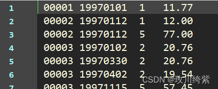
df.head()

# 数据中是否存储在缺失值
df.info()

RangeIndex: 69659 entries, 0 to 69658
Data columns (total 4 columns):#   Column         Non-Null Count  Dtype  
---  ------         --------------  -----  0   user_id        69659 non-null  int64  1   order_dt       69659 non-null  int64  2   order_product  69659 non-null  int64  3   order_amount   69659 non-null  float64
dtypes: float64(1), int64(3)
memory usage: 2.1 MB

# 将order_dt转换成时间类型
df['order_dt'] = pd.to_datetime(df['order_dt'], format='%Y%m%d')
df.info()

RangeIndex: 69659 entries, 0 to 69658
Data columns (total 4 columns):#   Column         Non-Null Count  Dtype         
---  ------         --------------  -----         0   user_id        69659 non-null  int64         1   order_dt       69659 non-null  datetime64[ns]2   order_product  69659 non-null  int64         3   order_amount   69659 non-null  float64       
dtypes: datetime64[ns](1), float64(1), int64(2)
memory usage: 2.1 MB

# 查看数据的统计描述
df.describe()

# 基于order_dt取出其中的月份
df['order_dt'].astype('datetime64[M]')
# 在源数据中添加一列表示月份:astype('datetime64[M]')
df['month'] = df['order_dt'].astype('datetime64[M]')
df.head()

第二部分：按月数据分析

• 用户每月花费的总金额
  • 绘制曲线图展示
• 所有用户每月的产品购买量
• 所有用户每月的消费总次数
• 统计每月的消费人数

# 用户每月花费的总金额
df.groupby(by='month')['order_amount'].sum()

month
1997-01-01    299060.17
1997-02-01    379590.03
1997-03-01    393155.27
1997-04-01    142824.49
1997-05-01    107933.30
1997-06-01    108395.87
1997-07-01    122078.88
1997-08-01     88367.69
1997-09-01     81948.80
1997-10-01     89780.77
1997-11-01    115448.64
1997-12-01     95577.35
1998-01-01     76756.78
1998-02-01     77096.96
1998-03-01    108970.15
1998-04-01     66231.52
1998-05-01     70989.66
1998-06-01     76109.30
Name: order_amount, dtype: float64

# plt.plot(df.groupby(by='month')['order_amount'].sum())
df.groupby(by='month')['order_amount'].sum().plot()

# 所有用户每月的产品购买量
df.groupby(by='month')['order_product'].sum()  #.plot()

month
1997-01-01    19416
1997-02-01    24921
1997-03-01    26159
1997-04-01     9729
1997-05-01     7275
1997-06-01     7301
1997-07-01     8131
1997-08-01     5851
1997-09-01     5729
1997-10-01     6203
1997-11-01     7812
1997-12-01     6418
1998-01-01     5278
1998-02-01     5340
1998-03-01     7431
1998-04-01     4697
1998-05-01     4903
1998-06-01     5287
Name: order_product, dtype: int64

# 所有用户每月的消费总次数（原始数据中的一行数据表示一次消费记录）
df.groupby(by='month')['user_id'].count()

month
1997-01-01     8928
1997-02-01    11272
1997-03-01    11598
1997-04-01     3781
1997-05-01     2895
1997-06-01     3054
1997-07-01     2942
1997-08-01     2320
1997-09-01     2296
1997-10-01     2562
1997-11-01     2750
1997-12-01     2504
1998-01-01     2032
1998-02-01     2026
1998-03-01     2793
1998-04-01     1878
1998-05-01     1985
1998-06-01     2043
Name: user_id, dtype: int64

# 统计每月的消费人数（可能一个月一个用户会消费多次，这时算一个人）nunique()表示统计去重后的个数
df.groupby(by='month')['user_id'].nunique()

month
1997-01-01    7846
1997-02-01    9633
1997-03-01    9524
1997-04-01    2822
1997-05-01    2214
1997-06-01    2339
1997-07-01    2180
1997-08-01    1772
1997-09-01    1739
1997-10-01    1839
1997-11-01    2028
1997-12-01    1864
1998-01-01    1537
1998-02-01    1551
1998-03-01    2060
1998-04-01    1437
1998-05-01    1488
1998-06-01    1506
Name: user_id, dtype: int64

第三部分：用户个体消费数据分析

• 用户消费总金额和消费总次数的统计描述
• 用户消费金额和消费产品数量的散点图
• 各个用户消费总金额的直方分布图(消费金额在1000之内的分布)
• 各个用户消费的总数量的直方分布图(消费商品的数量在100次之内的分布)

# 用户消费总金额和消费总次数的统计描述
df.groupby(by='user_id')['order_amount'].sum()  #总金额

user_id
1         11.77
2         89.00
3        156.46
4        100.50
5        385.61...  
23566     36.00
23567     20.97
23568    121.70
23569     25.74
23570     94.08
Name: order_amount, Length: 23570, dtype: float64

df.groupby(by='user_id')['order_dt'].count()  #总次数

user_id
1         1
2         2
3         6
4         4
5        11..
23566     1
23567     1
23568     3
23569     1
23570     2
Name: order_dt, Length: 23570, dtype: int64

# 用户消费金额和消费产品数量的散点图
user_amount_sum = df.groupby(by='user_id')['order_amount'].sum()
user_product_sum = df.groupby(by='user_id')['order_product'].sum()
plt.scatter(user_product_sum, user_amount_sum)

# 各个用户消费总金额的直方分布图(要求消费总金额在1000之内的分布)
df.groupby(by='user_id').sum().query('order_amount<=1000')['order_amount']
df.groupby(by='user_id').sum().query('order_amount<=1000')['order_amount'].hist()

# 各个用户消费的总数量的直方分布图(消费商品的数量在100次之内的分布)
df.groupby(by='user_id').sum().query('order_product<=100')['order_product'].hist()

第四部分：用户消费行为分析

• 用户第一次消费的月份分布，和人数统计
  • 绘制线形图
• 用户最后一次消费的时间分布，和人数统计
  • 绘制线形图
• 新老客户的占比
  • 消费一次为新用户
  • 消费多次为老用户
    • 分析出每一个用户的第一个消费和最后一次消费的时间
      • agg([‘func1’,‘func2’]):对分组后的结果进行指定聚合
    • 分析出新老客户的消费比例
• 用户分层
  • 分析得出每个用户的总购买量和总消费金额and最近一次消费的时间的表格rfm
  • RFM模型设计
    • R表示客户最近一次交易时间的间隔。
      • /np.timedelta64(1,‘D’)：去除days
    • F表示客户购买商品的总数量,F值越大，表示客户交易越频繁，反之则表示客户交易不够活跃。
    • M表示客户交易的金额。M值越大，表示客户价值越高，反之则表示客户价值越低。
    • 将R，F，M作用到rfm表中
  • 根据价值分层，将用户分为：
    • 重要价值客户
    • 重要保持客户
    • 重要挽留客户
    • 重要发展客户
    • 一般价值客户
    • 一般保持客户
    • 一般挽留客户
    • 一般发展客户
      • 使用已有的分层模型即可rfm_func

# 用户第一次消费的月份分布，和人数统计 绘制线形图
# 第一次消费的月份：每一个用户消费月份的最小值
df.groupby(by='user_id')['month'].min()

user_id
1       1997-01-01
2       1997-01-01
3       1997-01-01
4       1997-01-01
5       1997-01-01...    
23566   1997-03-01
23567   1997-03-01
23568   1997-03-01
23569   1997-03-01
23570   1997-03-01
Name: month, Length: 23570, dtype: datetime64[ns]

df.groupby(by='user_id')['month'].min().value_counts()  #人数统计
df.groupby(by='user_id')['month'].min().value_counts().plot()

# 用户最后一次消费的时间分布，和人数统计 绘制线形图
# 最后消费的月份：每一个用户消费月份的最大值
df.groupby(by='user_id')['month'].max().value_counts().plot()

# 新老客户的占比: 消费一次为新用户 消费多次为老用户
#如何获知用户是否为第一次消费？可以根据用户的消费时间进行判定
#如果用户的第一次消费时间和最后一次消费时间一样，则该用户只消费了一次为新用户，否则为老用户
new_old_user_df = df.groupby(by='user_id')['order_dt'].agg(['min', 'max'])  # agg(['func1','func2']):对分组后的结果进行多种指定聚合
new_old_user_df['min'] == new_old_user_df['max']  #True新用户，False老用户
# 统计true和false的个数
(new_old_user_df['min'] == new_old_user_df['max']).value_counts()

True     12054
False    11516
dtype: int64

# 用户分层
#     - 分析得出每个用户的总购买量和总消费金额and最近一次消费的时间的表格rfm
#     - RFM模型设计
#         - R表示客户最近一次交易时间的间隔。
#             - /np.timedelta64(1,'D')：去除days
#         - F表示客户购买商品的总数量,F值越大，表示客户交易越频繁，反之则表示客户交易不够活跃。
#         - M表示客户交易的金额。M值越大，表示客户价值越高，反之则表示客户价值越低。
#         - 将R，F，M作用到rfm表中
rfm = df.pivot_table(index='user_id', aggfunc={'order_product': 'sum', 'order_amount': 'sum', 'order_dt': 'max'})
rfm.head()

# R表示客户最近一次交易时间的间隔
max_dt = df['order_dt'].max()  # 所有数据中的最大日期
rfm['R'] = (max_dt - rfm['order_dt']) / np.timedelta64(1, 'D')  # /np.timedelta64(1,'D')：去除数据中的"days"
rfm.head()

# 去除多余的日期列
rfm.drop(labels='order_dt', axis=1, inplace=True)
rfm

23570 rows × 3 columns

rfm.columns = ['M', 'F', 'R']  #改变列名
rfm.head()

def rfm_func(x):# 存储的是三个字符串形式的0或者1level = x.map(lambda x: '1' if x >= 0 else '0')label = level.R + level.F + level.Md = {'111': '重要价值客户','011': '重要保持客户','101': '重要挽留客户','001': '重要发展客户','110': '一般价值客户','010': '一般保持客户','100': '一般挽留客户','000': '一般发展客户'}result = d[label]return result

#df.apply(func):可以对df中的行或者列进行某种（func）形式的运算
rfm['label'] = rfm.apply(lambda x: x - x.mean()).apply(rfm_func, axis=1)
rfm.head()

第五部分：用户的生命周期

• 将用户划分为活跃用户和其他用户
  • 统计每个用户每个月的消费次数
  • 统计每个用户每个月是否消费，消费记录为1否则记录为0
    • 知识点：DataFrame的apply和applymap的区别
      • applymap:返回df
      • 将函数做用于DataFrame中的所有元素(elements)
      • apply:返回Series
      • apply()将一个函数作用于DataFrame中的每个行或者列
  • 将用户按照每一个月份分成：
    • unreg:观望用户（前两月没买，第三个月才第一次买,则用户前两个月为观望用户）
    • unactive:首月购买后，后序月份没有购买则在没有购买的月份中该用户的为非活跃用户
    • new:当前月就进行首次购买的用户在当前月为新用户
    • active:连续月份购买的用户在这些月中为活跃用户
    • return:购买之后间隔n月再次购买的第一个月份为该月份的回头客

# 统计每个用户每个月的消费次数
user_month_count_df = df.pivot_table(index='user_id', values='order_dt', aggfunc='count', columns='month').fillna(0)
user_month_count_df.head()

#统计每个用户每个月是否消费，消费记录为1否则记录为0
df_purchase = user_month_count_df.applymap(lambda x: 1 if x >= 1 else 0)
df_purchase.head()

#将df_purchase中的原始数据0和1修改为new，unactive......,返回新的df叫做df_purchase_new
#固定算法
def active_status(data):status = []#某个用户每一个月的活跃度for i in range(18):#若本月没有消费if data[i] == 0:if len(status) > 0:if status[i-1] == 'unreg':status.append('unreg')else:status.append('unactive')else:status.append('unreg')#若本月消费else:if len(status) == 0:status.append('new')else:if status[i-1] == 'unactive':status.append('return')elif status[i-1] == 'unreg':status.append('new')else:status.append('active')return status

pivoted_status = df_purchase.apply(active_status,axis = 1)
pivoted_status.head()

user_id
1    [new, unactive, unactive, unactive, unactive, ...
2    [new, unactive, unactive, unactive, unactive, ...
3    [new, unactive, return, active, unactive, unac...
4    [new, unactive, unactive, unactive, unactive, ...
5    [new, active, unactive, return, active, active...
dtype: object

# pivoted_status.values.tolist()

# 填充回去
df_purchase_new = DataFrame(data=pivoted_status.values.tolist(),index=df_purchase.index,columns=df_purchase.columns)
df_purchase_new.head()

• 每月【不同活跃】用户的计数
  • purchase_status_ct = df_purchase_new.apply(lambda x : pd.value_counts(x)).fillna(0)
  • 转置进行最终结果的查看

purchase_status_ct = df_purchase_new.apply(lambda x : pd.value_counts(x)).fillna(0)
purchase_status_ct

# 转置：美观
purchase_status_ct.T

参考视频：【2022年张晓波亲授【数据分析自学课程】它来了！必备的Excel/SQL/Tableau/Python/数据黑话数据分析启蒙免费课程教程】 https://www.bilibili.com/video/BV1Bi4y1m7k7/?p=29&share_source=copy_web&vd_source=1170c577d779798202386e1f343fe38b

本文来自互联网用户投稿，文章观点仅代表作者本人，不代表本站立场，不承担相关法律责任。如若转载，请注明出处。 如若内容造成侵权/违法违规/事实不符，请点击【内容举报】进行投诉反馈！