【OpenCFD学习】二维钝锥

2023-10-26 08:34:18

文章目录

案例说明
- 运行方法
代码理解
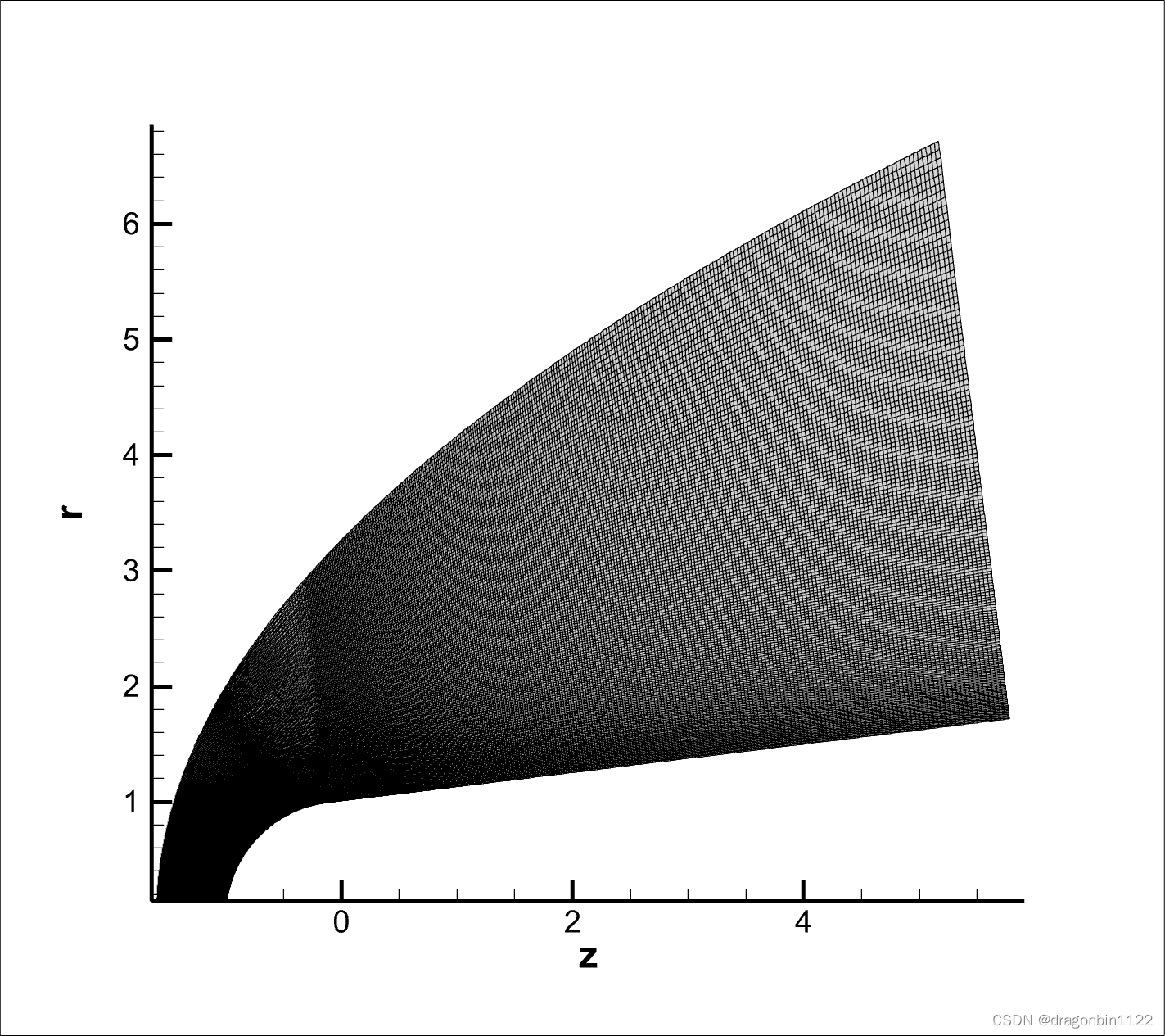
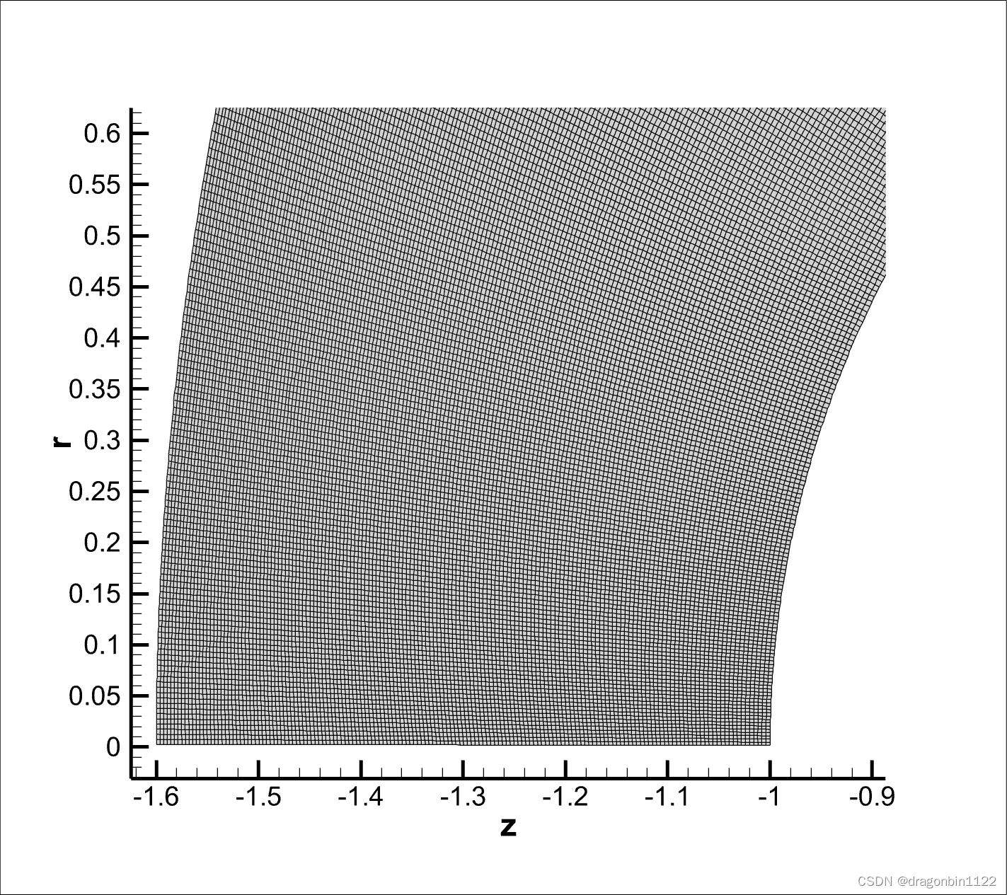
- 网格生成
- - 1. 网格控制文件
  - 2. 网格生成文件
- 流场读取
参考

案例说明

李新亮老师网盘：https://pan.baidu.com/s/1slfC5Yl
案例：OpenCFD-2D-cases/SC2d/bluentcone2d/

运行方法

生成网格和初值：cone2d0.dat、grid.dat、OCFD2d-Jacobi.dat、grid1d.dat、ss.dat、sx.dat、yb.dat

ifort mesh-withleading-3.0.f90 -o mesh-withleading
./mesh-withleading

链接初值和配置文件到opencfd2d-1.5.5.out。==初始阶段，受初值影响，计算容易发散，采用较小的时间步长及较低的 Reynolds 数，待算过一段时间后，再将计算参数恢复正常。==故先用 opencfd2d-1.in

ln -s cone2d0.dat opencfd2d.dat
ln -s opencfd2d-1.in opencfd2d.in

运行，10000步后程序停止，用slurm提交作业，vim bluntcone2d.sh

#!/bin/bash
#SBATCH -N 1
#SBATCH -n 20
mpirun -n 20 ./opencfd2d-1.5.5.out

sbatch -p G1Part_sce bluntcone2d.sh
tail -f slurm-xxx.out # 查看实时日志，xxx为作业号
sacct -D -X -j jobnum # 查看作业信息

注：mpirun的可执行文件要加./
4. 重新链接新的文件到opencfd2d-1.5.5.out

rm opencfd2d.in opencfd2d.dat
ln -s OCFD2d-0010000.dat opencfd2d.dat
ln -s opencfd2d-2.in opencfd2d.in

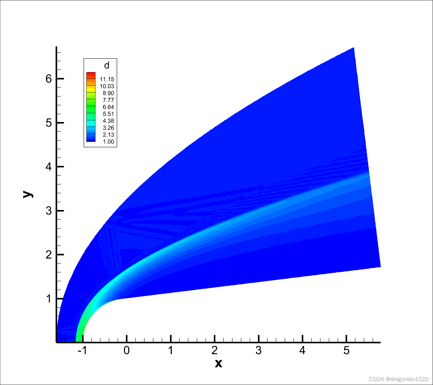
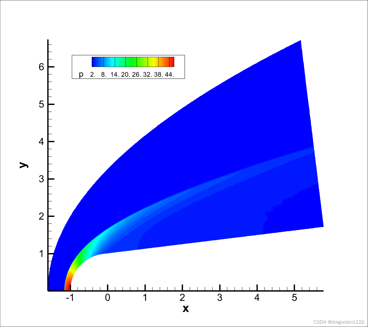
再次运行opencfd2d-1.5.5.out。到t=100耗时约10分钟。
后处理，生成flow2d.dat。弓形激波外的密度有点扰动，不知道对不对。

rm opencfd2d.dat
ln –s OCFD2d-0100000.dat opencfd2d.dat
ifort read-flow2d-v1.3.f90 -o read-flow2d
./read-flow2d

代码理解

网格生成

1. 网格控制文件

# 2d grid-generate control file  V3.0
#  nx     ny500    160
#  r1         seta1          b2       d2      seta21.0         7.            0.15    -1.6      20.
# x_end     alfax   nx_buff  alfax_buff  nxconjuction5.       2.5       20         1.002             10
#  Mesh_Y_TYPE deltyw_begin  deltyw_end     alfay1   alfay22      0.004              0.01         0.6      3.0

行数	变量	作用
1	nx	流向网格数
_	ny	法向网格数
2	r1	头部半径
_	seta1	半锥角( $^{\circ}$ )
_	b2、d2	计算网格外边界型线前半部分，抛物线， $z=b_2r^2+d_2$
_	seta2	计算网格外边界型线后半部分，直线，倾角为seta2
3	x_end	钝锥计算区长度
_	alfax	流向网格变化率，增大该值网格会更集中于钝锥头部
_	nx_buff	流向网格缓冲区（接近出口的区域）的网格数目
_	alfax_buff	流向缓冲区的网格延伸率
_	nxconjuction	连接点过渡区的网格数
4	Mesh_Y_TYPE	法向网格的类型，指数拉伸网格： $y=A(e^{\alpha\xi}-1)$
_	Mesh_Y_TYPE=1	$\alpha$ 在alfay1到alfay2之间均匀过渡
_	Mesh_Y_TYPE=2	指定第1层网格到壁面的距离，该距离从detlyw_begin(头部)到deltyw_end(尾部)均匀过渡

2. 网格生成文件

mesh-withleading-3.0.f90：程序结构：
- 网格配置文件.in读取
- 计算域内边界和外型线
- getsx()：计算流向指数拉伸坐标
- 计算内弧线上一点与钝头圆心的连线的延长线与外型线的相交位置：(xs,ys)为外型线的抛物线与直线交点；(xa,ya)为内弧线上的点；(xb,yb)为内弧线对应的外型线上的点
- simpson()：simpson积分计算外型线弧长，funs弧长公式：
  $ds=\sqrt{(dx)^2+(dy)^2}=\sqrt{1+(\frac{dy}{dx})^2}dx=\sqrt{1+(y')^2}dx$ $s=\int ds=\int\sqrt{1+(y')^2}dx$ $\int_a^bf(x)dx\approx\frac{h}{3}[f(x_0)+f(x_n)+4\sum_{i=1}^{n/2}f(x_{2i}-1)+2\sum_{i=1}^{n/2-1}f(x_{2i})]$ h=(b-a)/n，n 是子区间数目，且为偶数
- adjust_outer()：用三次函数让连接点光滑过渡
- get_y_form_ss()：牛顿迭代，找到连接点调整后的弧长对应的y坐标，之后即可确定对应x坐标
- getsy_V1()、getsy_V2()：两种类型网格拉伸
- get_Jacobian()：求Jacobian系数，生成初值
  - dx0、dy0：求导
注：
- 代码采用隐式声明implicit doubleprecision (a-h,o-z)，要确保全局变量common在这个范围内才有效声明

! mesh generator V 3.0 ,  blunted cone with small head-radius
! outline is a parabolic line conjucted with a linear line
! New feature of V2.0:
! destance between wall to the first mesh is constant and are given in control file
! Continues mesh step between conjuction point ( between cone and body ).
! New feature of V3.0:
! Step of the first mesh to the wall can be adjust by user. (linear function for hy1 (i=1) to hy2 (i=Ny) )
! IF IFLAG_MESHY_TYPE==1, V1.0 TYPE mesh, 2: V2.0 type mesh
!--------------------------------------------------------------
implicit doubleprecision (a-h,o-z)
real*8,parameter:: PI=3.1415926535897932
real*8,allocatable:: sx(:),sy(:,:),xa(:),xb(:), ya(:),yb(:),SL(:),delty(:)
real*8,allocatable:: ss(:),ss_new(:),xb_new(:),yb_new(:)
real*8,allocatable:: xx(:,:),yy(:,:)
common /para/ b2,d2,seta2,ys ! 注意：隐式声明的变量是否在a-h,o-z的范围open(66,file='grid2d-withleading.in') ! 读取网格配置文件
read(66,*)
read(66,*)
read(66,*) nx,ny
read(66,*)
read(66,*) r1,seta1,b2,d2,seta2
read(66,*)
! read(66,*) S0, alfay
read(66,*) x_end, alfax, nx_buff, alfax_buff, nxconjunction_buffer
read(66,*)
read(66,*) IFLAG_MESHY_TYPE, deltyw_i_begin, deltyw_i_end,alfay1,alfay2
read(66,*)
close(66)allocate(sx(nx),sy(nx,ny),xa(nx),xb(nx),  &
ya(nx),yb(nx),SL(nx),delty(nx),xx(nx,ny),yy(nx,ny), &
ss(nx),ss_new(nx),xb_new(nx),yb_new(nx))!c-------------------------------计算域内边界和外型线
seta1=seta1*PI/180.d0
seta2=seta2*PI/180.d0ys=1.d0/(2.d0*b2*tan(seta2)) ! 外型线：抛物线与直线相交处y坐标，斜率相等
xs=b2*ys*ys+d2
ds=1.d0/(nx-1.d0)
SL0=(PI/2.-seta1)*r1+(x_end+r1*sin(seta1))/cos(seta1) ! 钝锥表面弧长：曲线+直线!--------------------------------------------------
if(IFLAG_MESHY_TYPE .eq. 1) thenprint*, "V1.0 type y-mesh "
else if ( IFLAG_MESHY_TYPE .eq. 2) thenprint*, "V2.0 type y-mesh, the first step to the wall is given !"
endif
!--------------------------------------------------call getsx(nx,nx_buff,sx,alfax,alfax_buff) ! 流向拉伸坐标
!c ---------------------------do i=1,nxs=sx(i)*SL0if(s .le. (PI/2.-seta1)*r1) then ! 钝锥头部圆弧上，弧长转为直角坐标alfa=s/r1xa(i)=-r1*cos(alfa)ya(i)=r1*sin(alfa)! (xb,yb) is the coordination of the outline
! (xb,yb) is located on the parabolic line
! (xa,ya)与锥头圆心连线延长线与外型线的抛物线的交点
! xb=b2*yb**2+d2; yb/(-xb)=tan(alfa) => 联立，求根公式xb(i)=(1.-sqrt(1.-4.*b2*d2*tan(alfa)**2))/(2.*b2*tan(alfa)**2)yb(i)=-xb(i)*tan(alfa)if(xb(i) .gt. xs) then ! 延长线与外型线交于直线部分
! (xb,yb) is located on the linear line
! (yb-ys)/(xb-xs)=tan(seta2); yb/(-xb)=tan(alfa) => 联立xb(i)=-(ys-tan(seta2)*xs)/(tan(alfa)+tan(seta2))yb(i)=-tan(alfa)*xb(i)endif
!    	 if(alfa .le. PI/2.-seta2) then
!            xb(i)=-r2*cos(alfa)
!            yb(i)=r2*sin(alfa)
!        else
!            xb(i)=-(y3-tan(seta2)*x3)/(tan(alfa)+tan(seta2))
!            yb(i)=-tan(alfa)*xb(i)
!            yb(i)=y3+tan(seta2)*(xb(i)-x3)
!        endifelse ! 内弧线的直线部分sa=s-(PI/2.-seta1)*r1xa(i)=-r1*sin(seta1)+sa*cos(seta1) ! 内弧直线上一点转直角坐标ya(i)=r1*cos(seta1)+sa*sin(seta1)! 内弧直线的垂线与外型线抛物线相交! xb=b2*yb**2+d2; (xa-xb)/(yb-ya)=tan(seta1); 联立，求根公式at=b2 bt=tan(seta1)ct=d2-xa(i)-ya(i)*tan(seta1)yb(i)=(-bt+sqrt(bt*bt-4.*at*ct))/(2.*at)xb(i)=b2*yb(i)*yb(i)+d2! 内弧直线的垂线与外型线的直线相交! (xa-xb)/(yb-ya)=tan(seta1); (yb-ys)/(xb-xs)=tan(seta2);if(xb(i) .gt. xs) then xb(i)=(ya(i)-ys+tan(seta2)*xs-tan(PI/2.+seta1)*xa(i))/   &(tan(seta2)-tan(PI/2.+seta1))yb(i)=ys+tan(seta2)*(xb(i)-xs)endifendifcall simpson (ss(i),0.d0,yb(i))     ! The arc length of outter-line
enddo
!--------The point nearest to the conjcetion point
do i=1,nxs=sx(i)*SL0if(s .gt. (PI/2.-seta1)*r1) theni_conjunction=igoto 101endif
enddo
101   continue
print*, i_conjunction
!-------------------
! Adjuct mesh points near to the conjunction points
call adjust_outter(nx,ss,ss_new,i_conjunction,nxconjunction_buffer)do i=1,nxcall get_y_form_ss(ss_new(i),yb_new(i),1.d0)
enddoopen(33,file='yb.dat')
do i=2,nxwrite(33,'(6f16.8)') i*1., yb(i), yb_new(i)
enddodo i=1,nxif(yb_new(i) .lt. ys) then   ! located on the parabolic linexb_new(i)=b2*yb_new(i)**2 + d2elsexb_new(i)= xs + (yb_new(i)-ys)/tan(seta2)endif
enddoopen(55,file="grid1d.dat")
do i=1,nxwrite(55,"(4f15.6)") xb(i),yb(i),xb_new(i),yb_new(i)
enddo
close(55)
!----------------------------------------------
xb=xb_new
yb=yb_new
!c----------------------------if(IFLAG_MESHY_TYPE .eq. 2) thendo i=1,nxSL(i)=sqrt((xa(i)-xb(i))**2+(ya(i)-yb(i))**2)delty(i)=deltyw_i_begin+(deltyw_i_end- deltyw_i_begin)*(i-1.d0)/(nx-1.d0)enddocall getsy_V2(nx,ny,sy,SL,delty)
elsecall getsy_V1(nx,ny,sy,alfay1,alfay2)
endifdo i=1,nxdo j=1,nyxx(i,j)=xb(i)+(xa(i)-xb(i))*sy(i,j)yy(i,j)=yb(i)+(ya(i)-yb(i))*sy(i,j)enddo
enddo!------------------------------------------------
! Warning , following code maybe have some problems ...
! goto 300! Adjust mesh between i_conjunction
!         n2=nxconjunction_buffer/2
!     do i=i_conjunction-n2,i_conjunction+n2
!             alfa=acos(xa(i)/r1)
!         if(alfa .le. PI/2.d0+seta1) alfa= PI/2.d0+seta1
!         call get_coe1(a,b,c,d,xa(i),ya(i),xb(i),yb(i),tan(alfa))
!         call simpson1 (s,xa(i),xb(i),a,b,c,d)
!         do j=1,ny
!             s1=s*sy(i,j)
!                 call get_y_form_ss1(s1,x, xb(i),a,b,c,d)
!             xx(i,j)=x
!             yy(i,j)=a*xx(i,j)**3+b*xx(i,j)**2+c*xx(i,j)+d
!             enddo
!         enddo
!300 continue!-------------------------------------------------call get_Jacobian(nx,ny,yy,xx)end!----------------------------------------------------------------------------!c======== x direction ------------------
subroutine getsx(nx,nx_buff,sx,alfax,alfax_buff) ! 流向坐标拉伸implicit doubleprecision (a-h,o-z)dimension sx(nx)nx1=nx-nx_buffdx=1.d0/(nx1-1.d0)A=1.d0/(exp(alfax)-1.d0)do i=1,nx1s=(i-1./2.)*dxsx(i)=A*(exp(s*alfax)-1.d0)enddodo i=nx1+1,nxsx(i)=sx(i-1)+alfax_buff*(sx(i-1)-sx(i-2))enddoopen(55,file="sx.dat")do k=1,nx-1write(55,*) k, sx(k),sx(k+1)-sx(k)enddo
end!c================================================================
subroutine get_Jacobian(nx,ny,xx,yy)implicit doubleprecision(a-h,o-z)parameter (LAP=3)dimension xx(nx,ny),yy(nx,ny)dimension Akx(nx,ny),Aky(nx,ny), Aix(nx,ny),Aiy(nx,ny), Ajac(nx,ny)dimension xk(nx,ny),xi(nx,ny),  yk(nx,ny),yi(nx,ny)dimension xx1(1-LAP:nx,ny),yy1(1-LAP:nx,ny)dimension d(nx,ny),u(nx,ny),v(nx,ny),T(nx,ny)hx=1.d0/(nx-1.d0)hy=1.d0/(ny-1.d0)do j=1,nydo i=1,nxxx1(i,j)=xx(i,j)yy1(i,j)=yy(i,j)enddoenddodo j=1,nydo i=1,LAPi1=1-ixx1(i1,j)=-xx(i,j)yy1(i1,j)=yy(i,j)enddoenddocall dx0(xx1,xk,nx,ny,hx,LAP)call dx0(yy1,yk,nx,ny,hx,LAP)call dy0(xx,xi,nx,ny,hy)call dy0(yy,yi,nx,ny,hy)Ajac=xk*yi-xi*ykAjac=1./AjacAkx=Ajac*yiAky=-Ajac*xiAix=-Ajac*ykAiy=Ajac*xkopen(55,file='OCFD2d-Jacobi.dat',form='unformatted')write(55) xxwrite(55) yywrite(55) Akxwrite(55) Akywrite(55) Aixwrite(55) Aiywrite(55) Ajacclose(55)do j=1,nydo i=1,nxif(Ajac(i,j).lt.1.e-5) print*, i,j,Ajac(i,j)enddoenddoopen(33,file='grid.dat')write(33,*) 'variables=z,r,Akx,Aky,Aix,Aiy,Ajac'write(33,*) 'zone i=',nx , 'j=',nydo j=1,nydo i=1,nxwrite(33,'(7f15.6)') yy(i,j),xx(i,j),Akx(i,j),Aky(i,j),   &Aix(i,j),Aiy(i,j),Ajac(i,j)enddoenddoclose(33)!  Generate initial data ...Istep=0tt=0.d=1.u=0.v=1.T=1.open(44,file='cone2d0.dat',form='unformatted')write(44) Istep,ttwrite(44) dwrite(44) uwrite(44) vwrite(44) Tclose(44)
end!c==================================================================
subroutine dx0(f,fx,nx,ny,hx,LAP)implicit doubleprecision (a-h,o-z)dimension f(1-LAP:nx,ny),fx(nx,ny)b1=8.d0/(12.d0*hx)b2=1.d0/(12.d0*hx)a1=1.d0/(60.d0*hx)a2=-3.d0/(20.d0*hx)a3=3.d0/(4.d0*hx)do j=1,nydo i=1,nx-3fx(i,j)=a1*(f(i+3,j)-f(i-3,j)) +a2*(f(i+2,j)-f(i-2,j)) +a3*(f(i+1,j)-f(i-1,j))enddoenddodo j=1,nyfx(nx-2,j)=b1*(f(nx-1,j)-f(nx-3,j)) -b2*(f(nx,j)-f(nx-4,j))fx(nx-1,j)=(f(nx-3,j)-6.d0*f(nx-2,j)+3.d0*f(nx-1,j) +2.d0*f(nx,j))/(6.d0*hx)fx(nx,j)=(f(nx-2,j)-4.d0*f(nx-1,j)+3.d0*f(nx,j))/(2.d0*hx)enddo
end!----------------------------------------------
subroutine dy0(f,fy,nx,ny,hy)implicit doubleprecision (a-h,o-z)dimension f(nx,ny),fy(nx,ny)b1=8.d0/(12.d0*hy)b2=1.d0/(12.d0*hy)a1=1.d0/(60.d0*hy)a2=-3.d0/(20.d0*hy)a3=3.d0/(4.d0*hy)do j=4,ny-3do i=1,nxfy(i,j)=a1*(f(i,j+3)-f(i,j-3)) +a2*(f(i,j+2)-f(i,j-2)) +a3*(f(i,j+1)-f(i,j-1))enddoenddodo i=1,nxfy(i,1)=(-3.d0*f(i,1)+4.d0*f(i,2)-f(i,3))/(2.d0*hy)fy(i,2)=(-2.d0*f(i,1)-3.d0*f(i,2)+6.d0*f(i,3)-f(i,4)) /(6.d0*hy)fy(i,3)=b1*(f(i,4)-f(i,2)) -b2*(f(i,5)-f(i,1))fy(i,ny-2)=b1*(f(i,ny-1)-f(i,ny-3))  -b2*(f(i,ny)-f(i,ny-4))fy(i,ny-1)=(f(i,ny-3)-6.d0*f(i,ny-2)+3.d0*f(i,ny-1)  +2.d0*f(i,ny))/(6.d0*hy)fy(i,ny)=(f(i,ny-2)-4.d0*f(i,ny-1)+3.d0*f(i,ny))/(2.d0*hy)enddo
end!-------------------------------------------------
! Mesh_Y_TYPE=1
subroutine getsy_V1(nx,ny,sy,alfay1,alfay2)implicit doubleprecision (a-h,o-z)dimension sy1(nx,ny),sy(nx,ny)dy=1.d0/(ny-1.d0)do i=1,nxalfay=alfay1+(i-1.d0)/(nx-1.d0)*(alfay2-alfay1)A=1.d0/(exp(alfay)-1.d0)do j=1,nys=(j-1.d0)*dysy1(i,j)=A*(exp(s*alfay)-1.d0)enddodo j=1,nyj1=ny+1-jsy(i,j)=sy1(i,ny)-sy1(i,j1)enddoenddo
end!-------------------------------------------------
! Mesh_Y_TYPE=1
!  generate a exp function:  y(j)=A*(exp(b*sj)-1)  while y(1)=0, y(ny)=SL and y(2)=deltx
!      sy=a(exp(b*s)-1)subroutine getsy_V2(nx,ny,sy,SL,deltx)implicit doubleprecision (a-h,o-z)dimension sy1(nx,ny),sy(nx,ny),SL(nx),deltx(nx)dy=1.d0/(ny-1.d0)b=3.5d0      ! initial datado i=1,nx
!---------------------------------------delta=deltx(i)/SL(i)
! using Newton method get coefficient
100     continue
!        fb=exp(b/(ny-1.d0))-1.d0-delta*(exp(b)-1.d0)
!            fbx=exp(b/(ny-1.d0))/(ny-1.d0)-delta*exp(b)fb=(exp(b/(ny-1.d0))-1.d0)/(exp(b)-1.d0)-deltafbx=(exp(b/(ny-1.d0))/(ny-1.d0)*(exp(b)-1.d0) - &(exp(b/(ny-1.d0))-1.d0)*exp(b)  )/((exp(b)-1.d0))**2bnew=b-fb/fbxif(abs(b-bnew) .gt. 1.d-6) thenb=bnewgoto 100endifb=bnewa=1.d0/(exp(b)-1.d0)do j=1,nys=(j-1.d0)*dysy1(i,j)=a*(exp(s*b)-1.d0)enddo
!-------------- revise -----------do j=1,nyj1=ny+1-jsy(i,j)=sy1(i,ny)-sy1(i,j1)enddoenddo
end!-------------------------------------------
!  simpson integral, the arc length of outer-line
subroutine simpson (s,xa,xb)implicit doubleprecision (a-h,o-z)integer,parameter:: nx=100dx=(xb-xa)/(nx-1.d0)s1=0.d0s2=0.d0do k=2,nxx=xa+(k-1.d0)*dx-dx/2.d0s1=s1+funs(x)enddodo k=2,nx-1x=xa+(k-1.d0)*dxs2=s2+funs(x)enddos=(funs(xa)+funs(xb)+4.d0*s1+2.d0*s2)*dx/6.d0
end!-------------------------------------------
! Outline: Arc length differentiation of parabola
function funs(x)implicit doubleprecision (a-h,o-z)common /para/ b,d, seta2,ys
!        funs=cos(x)
!    parabolic   y=b*x*x+dif(x .lt. ys) thenfuns=sqrt(1.d0+(2.d0*b*x)**2)        ! x is r  ; located in the parabolic lineelsefuns=1.d0/sin(seta2)    ! linearendif
end!---------------------------------------------
subroutine get_y_form_ss(sa,y,y0)implicit doubleprecision (a-h,o-z)real*8,parameter:: dx=0.001d0y=y0
100     continuecall simpson(s,0.d0,y)sy=funs(y)ynew=y-(s-sa)/syif(abs(y-ynew) .gt. 1.d-6) theny=ynewgoto 100endify=ynew
end!-------------------------------
function funs1(x,a,b,c,d)implicit doubleprecision (a-h,o-z)
!     y=a*x**3+b*x*x+c*x+dfuns1=sqrt(1.d0+(3.d0*a*x*x+2.d0*b*x+3.d0*c)**2) ! x is r; located in the parabolic line
end!-------------------------------
subroutine simpson1 (s,xa,xb,a,b,c,d)implicit doubleprecision (a-h,o-z)integer,parameter:: nx=100dx=(xa-xb)/(nx-1.d0)s1=0.d0s2=0.d0do k=2,nxx=xb+(k-1.d0)*dx-dx/2.d0s1=s1+funs1(x,a,b,c,d)enddodo k=2,nx-1x=xb+(k-1.d0)*dxs2=s2+funs1(x,a,b,c,d)enddos=(funs1(xa,a,b,c,d)+funs1(xb,a,b,c,d)+4.d0*s1+2.d0*s2)*dx/6.d0
end!---------------------------------------------
subroutine get_y_form_ss1(sa,y,yb,a,b,c,d)implicit doubleprecision (a-h,o-z)real*8,parameter:: dx=0.001d0y=yb
100     continuecall simpson1(s,y,yb,a,b,c,d)sy=funs1(y,a,b,c,d)ynew=y-(s-sa)/syif(abs(y-ynew) .gt. 1.d-6) theny=ynewgoto 100endify=ynew
end!--------------------------------------------
! Adjust the grid of the outer boundary to ensure a smooth transition of arc length spacing near the connection point
! Use Cubic function for transition
subroutine adjust_outter(nx,ss,ss_new,i_conjunction,nxconjunction_buffer)implicit doubleprecision (a-h,o-z)real*8 ss(nx),ss_new(nx)ss_new=ssn2=nxconjunction_buffer/2ia=i_conjunction-n2ib=i_conjunction+n2det1=ss(ia)-ss(ia-1)det2=ss(ib+1)-ss(ib)ds=1.d0/(2.d0*n2)do i=1,2*n2+1s=(i-1.d0)*dsxh0=(1.d0+2.d0*s)*(s-1.d0)**2xh1=(1.d0+2.d0*(1.d0-s))*s*sxhf0=s*(s-1.d0)**2xhf1=(s-1.d0)*s*sss_new(i+ia-1)=ss(ia)*xh0+ss(ib)*xh1+det1/ds*xhf0+det2/ds*xhf1enddoopen(55,file="ss.dat")do k=2,nxwrite(55,"(I3,4f16.8)") k, ss(k),ss_new(k), ss(k)-ss(k-1),  &ss_new(k)-ss_new(k-1)enddo
end
!----------------------
! cubic function y =a*x**3+b*x**2+c*x+d, so that y(xa)=ya, y(xb)=yb, y'(xa)=ska, y"(xb)=0
subroutine get_coe1(a,b,c,d,xa,ya,xb,yb,ska)implicit doubleprecision (a-h,o-z)a=(yb-ya-ska*(xb-xa))/(2.d0*xa**3+6.d0*xa*xb*xb  &-6.d0*xa*xa*xb-2.d0*xb**3)b=-3.d0*xb*ac=ska+a*(-3*xa*xa+6.d0*xa*xb)d=ya-ska*xa+a*(2.d0*xa**3-3.d0*xa*xa*xb)
end
!------------------------

流场读取

read-flow2d-v1.3.f90：读取配置文件、网格信息，保存数据为tecplot格式

! read-flow2d  ver 1.3implicit doubleprecision (a-h,o-z)
real*8,allocatable,dimension(:,:):: d,u,v,T,rr,zz
real*8 tt
integer istep
!-----------------------------------------
gamma=1.4d0
open(33,file="opencfd2d.in")
do k=1,4read(33,*)
enddo
read(33,*) nx,ny
close(33)allocate(rr(nx,ny),zz(nx,ny))
allocate(d(nx,ny),u(nx,ny),v(nx,ny),T(nx,ny))
!------------------------------------------------------
PI=3.14159265358979d0!---------read grid message --------------------------
open(66,file="OCFD2d-Jacobi.dat",form="unformatted")
read(66) rr
read(66) zz
close(66)seta0=atan( (rr(nx,ny)-rr(nx-1,ny)) / (zz(nx,ny)-zz(nx-1,ny)) )
print*, "cone angle  (degree) =" , seta0*180.d0/PI!---------read data file------------------------
open(33,file="opencfd2d.dat",form="unformatted")
read(33) Istep,tt
read(33) d
read(33) u
read(33) v
read(33) T
close(33)print*, "read data OK ..."
print*, "Istep,tt=",Istep,ttopen(44,file="flow2d.dat")
write(44,*) "variables=x,y,d,ur,uz,T,p,s"
write(44,*) "zone i= ",nx, " j= ",nydo j=1,nydo i=1,nxwrite(44,"(9f15.6)") zz(i,j),rr(i,j),d(i,j),u(i,j),v(i,j),  &T(i,j), d(i,j)*T(i,j), T(i,j)*d(i,j)/d(i,j)**gammaenddo
enddo
close(44)deallocate(rr,zz,d,u,v,T)
!--------------------------------------------------
end

参考

https://blog.csdn.net/qq_42988706/article/details/131412355
https://blog.csdn.net/qq_42988706/article/details/131539461
OpenCFD使用手册、理论手册
OpenCFD2d教学示例》

本文来自互联网用户投稿，文章观点仅代表作者本人，不代表本站立场，不承担相关法律责任。如若转载，请注明出处。 如若内容造成侵权/违法违规/事实不符，请点击【内容举报】进行投诉反馈！

标签：技术

上一篇 > OPENGL（ubuntu下的实践）——基础篇
下一篇 > Microsoft .NET Framework 3.5 安装失败，错误码：0x800f081f；

Duilib中list控件支持ctrl和shif多行选中的实现

[ICML2015]Batch Normalization:Accelerating Deep Network Training by Reducing Internal Covariate Shif

win10系统微软输入法于eclipse ctrl+shif+f冲突间接处理办法

Codeforces Round #259 (Div. 2) B. Little Pony and Sort by Shif

读LDD3，内存映射与DMA--PAGE_SHIF…

VMware虚拟机安装XP【要先分区，再设置BOOT 启动CD，shif+上移】

更换iBus五笔的左与右Shif

sublime ctrl+shif+f 没用解决办法

idea 对 ctrl + z 的撤销是 ctrl + shif + z

计算机最早的设计师应用于,计算机应用基础选择题doc.doc

win10自带截图神器：Win+Shift+S

Python基础之文件目录操作

python简述目录_Python基础之文件目录操作(示例代码)

tp5 如何做数据采集

任务2-7(服务器字体+阿里巴巴矢量库)

html标签（1)：h1~h6,p,br,pre,hr

TI 电量计介绍与芯片选型指南

几款TI电源芯片简介

TI DSP芯片C2000系列读取FLASH数据

德州仪器(Ti)平台嵌入式开发基础

TI三相电机智能栅极驱动芯片特点分类

省选模拟（12.08） T3 圈圈圈圈圈圈圈圈

Hadoop生态圈技术栈（上）

大数据开发基础入门与项目实战（三）Hadoop核心及生态圈技术栈之6.Impala交互式查询

小猿圈之Linux下Mysql 操作命令

大数据Hadoop生态圈常用面试题

大数据开发基础入门与项目实战（三）Hadoop核心及生态圈技术栈之4.Hive DDL、DQL和数据操作

备战Noip2018模拟赛11（B组）T3 Monogatari 物语

【智能优化算法-圆圈搜索算法】基于圆圈搜索算法Circle Search Algorithm求解单目标优化问题附matlab代码

NYOJ 78 圈水池

递归问题跑道汽车绕圈问题 Python实现

Hadoop生态圈（三）：MapReduce

【OpenCFD学习】二维钝锥

文章目录

案例说明

运行方法

代码理解

网格生成

1. 网格控制文件

2. 网格生成文件

流场读取

参考

相关文章