Neural Networks and Deep Learnging week4 Deep Neural Network - Application
该实验作业的主要目的
- 将刚刚完成的神经网络模块,组合到一起,并进行对猫片的分类
你可能感兴趣的文献
http://stackoverflow.com/questions/1907993/autoreload-of-modules-in-ipython 刚刚完成的模块很多,如何快速加载那些常用模块
总体进程
需要手写的就两部分,一个是初始化设定,另一个是整合上一作业的模块,功利的完成作业很快,为了更好的了解过程,建议按照指导的内容,全部过一遍,需要写代码的模块用***在开头标出
- 载入文件(各种会用到的头文件/包)
- 载入数据,并转换成可以处理格式——长期按照coursera在线的内容进行的坏处是,当自己做东西时,遇到各种格式的数据(比如excel读取数据,图片数据,原始数据都不是包的形式),发现很多东西不能直接用(比如shape,需要np.array(data)) coursera上的操作会让你膨胀
- 实现模块,已经在上一作业中完成,因而这个作业在开头进行了导入模块
- *** 2层神经网络的搭建,有两个东西绕不开,初始化超参量,整合模块
- *** L层神经网络的搭建,结果上,上下两个相同,但是意义不同,下面的这个更加独立、模块化
- 测试我们的神经网络
在需要写代码的前面我将提示任务目标
Deep Neural Network for Image Classification: Application
When you finish this, you will have finished the last programming assignment of Week 4, and also the last programming assignment of this course!
You will use the functions you'd implemented in the previous assignment to build a deep network, and apply it to cat vs non-cat classification. Hopefully, you will see an improvement in accuracy relative to your previous logistic regression implementation.
After this assignment you will be able to:
- Build and apply a deep neural network to supervised learning.
Let's get started!
1 - Packages
Let's first import all the packages that you will need during this assignment.
- numpy is the fundamental package for scientific computing with Python.
- matplotlib is a library to plot graphs in Python.
- h5py is a common package to interact with a dataset that is stored on an H5 file.
- PIL and scipy are used here to test your model with your own picture at the end.
- dnn_app_utils provides the functions implemented in the "Building your Deep Neural Network: Step by Step" assignment to this notebook.
- np.random.seed(1) is used to keep all the random function calls consistent. It will help us grade your work.
import time
import numpy as np
import h5py
import matplotlib.pyplot as plt
import scipy
from PIL import Image
from scipy import ndimage
from dnn_app_utils_v3 import *%matplotlib inline
plt.rcParams['figure.figsize'] = (5.0, 4.0) # set default size of plots
plt.rcParams['image.interpolation'] = 'nearest'
plt.rcParams['image.cmap'] = 'gray'%load_ext autoreload
%autoreload 2np.random.seed(1)
2 - Dataset
You will use the same "Cat vs non-Cat" dataset as in "Logistic Regression as a Neural Network" (Assignment 2). The model you had built had 70% test accuracy on classifying cats vs non-cats images. Hopefully, your new model will perform a better!
Problem Statement: You are given a dataset ("data.h5") containing:
- a training set of m_train images labelled as cat (1) or non-cat (0)
- a test set of m_test images labelled as cat and non-cat
- each image is of shape (num_px, num_px, 3) where 3 is for the 3 channels (RGB).
Let's get more familiar with the dataset. Load the data by running the cell below.
train_x_orig, train_y, test_x_orig, test_y, classes = load_data()The following code will show you an image in the dataset. Feel free to change the index and re-run the cell multiple times to see other images.
# Example of a picture
index = 10
plt.imshow(train_x_orig[index])
print ("y = " + str(train_y[0,index]) + ". It's a " + classes[train_y[0,index]].decode("utf-8") +  " picture.")
# Explore your dataset
m_train = train_x_orig.shape[0]
num_px = train_x_orig.shape[1]
m_test = test_x_orig.shape[0]print ("Number of training examples: " + str(m_train))
print ("Number of testing examples: " + str(m_test))
print ("Each image is of size: (" + str(num_px) + ", " + str(num_px) + ", 3)")
print ("train_x_orig shape: " + str(train_x_orig.shape))
print ("train_y shape: " + str(train_y.shape))
print ("test_x_orig shape: " + str(test_x_orig.shape))
print ("test_y shape: " + str(test_y.shape))As usual, you reshape and standardize the images before feeding them to the network. The code is given in the cell below.
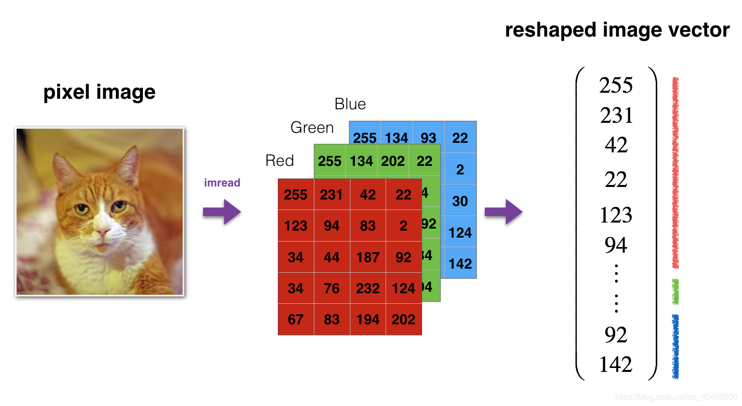
# Reshape the training and test examples
train_x_flatten = train_x_orig.reshape(train_x_orig.shape[0], -1).T   # The "-1" makes reshape flatten the remaining dimensions
test_x_flatten = test_x_orig.reshape(test_x_orig.shape[0], -1).T# Standardize data to have feature values between 0 and 1.
train_x = train_x_flatten/255.
test_x = test_x_flatten/255.print ("train_x's shape: " + str(train_x.shape))
print ("test_x's shape: " + str(test_x.shape))
12,288 equals 64×64×3 which is the size of one reshaped image vector.
3 - Architecture of your model
Now that you are familiar with the dataset, it is time to build a deep neural network to distinguish cat images from non-cat images.
You will build two different models:
- A 2-layer neural network
- An L-layer deep neural network
You will then compare the performance of these models, and also try out different values for LL.
Let's look at the two architectures.
3.1 - 2-layer neural network
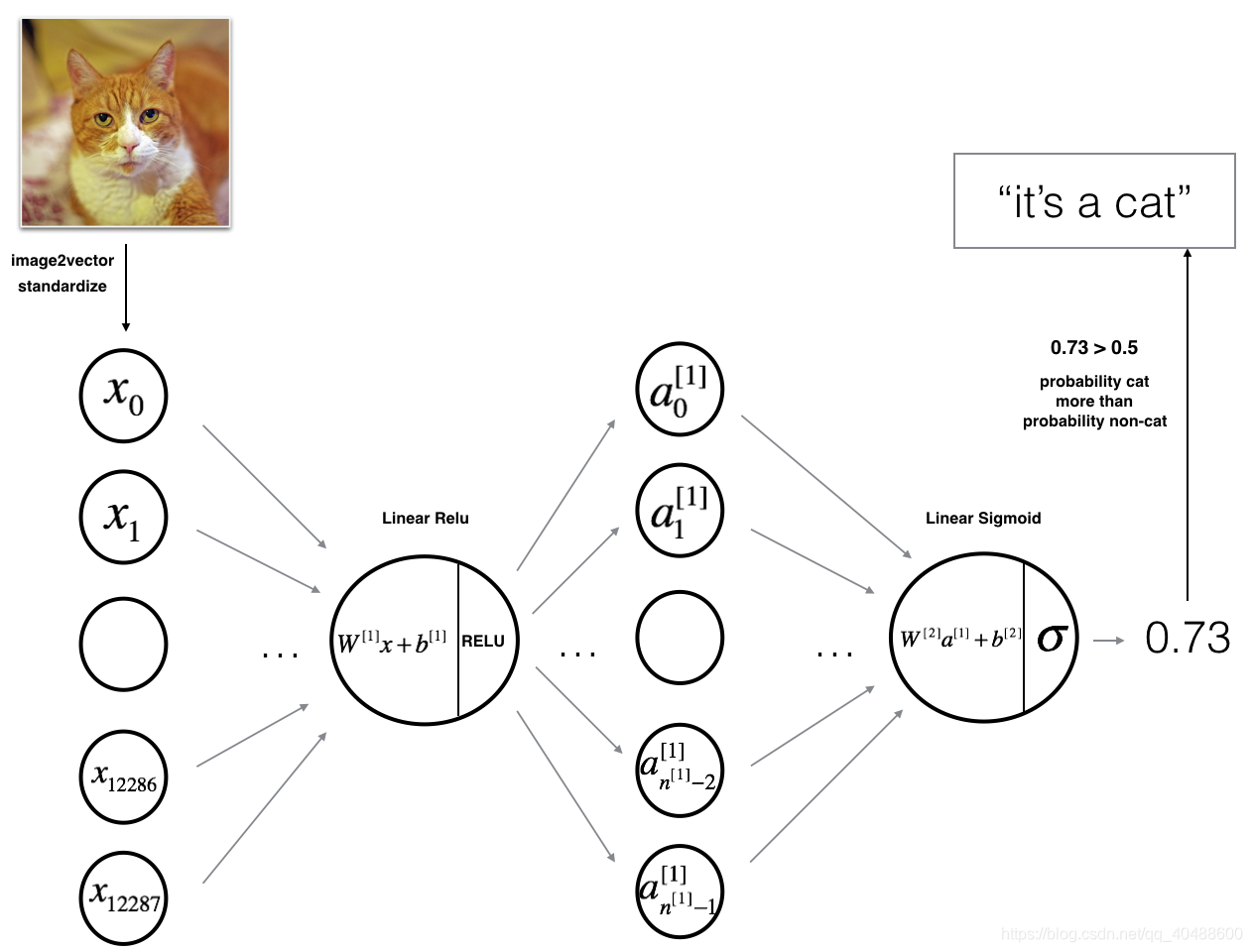
The model can be summarized as: INPUT -> LINEAR -> RELU -> LINEAR -> SIGMOID -> OUTPUT.
Detailed Architecture of figure 2:
- The input is a (64,64,3) image which is flattened to a vector of size (12288,1)(12288,1).
- The corresponding vector: [x0,x1,...,x12287]T is then multiplied by the weight matrix W[1] of size (n[1],12288).
- You then add a bias term and take its relu to get the following vector: [a[1]0,a[1]1,...,a[1]n[1]−1]T.
- You then repeat the same process.
- You multiply the resulting vector by W[2] and add your intercept (bias).
- Finally, you take the sigmoid of the result. If it is greater than 0.5, you classify it to be a cat.
3.2 - L-layer deep neural network
It is hard to represent an L-layer deep neural network with the above representation. However, here is a simplified network representation:
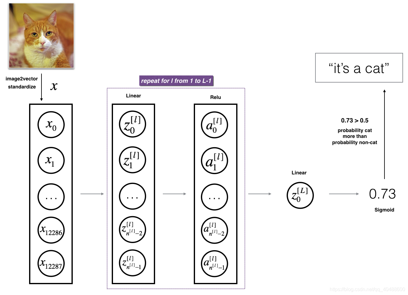
Detailed Architecture of figure 3:
- The input is a (64,64,3) image which is flattened to a vector of size (12288,1).
- The corresponding vector: [x0,x1,...,x12287]T[x0,x1,...,x12287]T is then multiplied by the weight matrix W[1]W[1] and then you add the intercept b[1]b[1]. The result is called the linear unit.
- Next, you take the relu of the linear unit. This process could be repeated several times for each (W[l],b[l])(W[l],b[l]) depending on the model architecture.
- Finally, you take the sigmoid of the final linear unit. If it is greater than 0.5, you classify it to be a cat.
3.3 - General methodology
As usual you will follow the Deep Learning methodology to build the model:
1. Initialize parameters / Define hyperparameters
2. Loop for num_iterations:a. Forward propagationb. Compute cost functionc. Backward propagationd. Update parameters (using parameters, and grads from backprop)
4. Use trained parameters to predict labels
Let's now implement those two models!
4 - Two-layer neural network
Question: Use the helper functions you have implemented in the previous assignment to build a 2-layer neural network with the following structure: LINEAR -> RELU -> LINEAR -> SIGMOID. The functions you may need and their inputs are:
def initialize_parameters(n_x, n_h, n_y):...return parameters
def linear_activation_forward(A_prev, W, b, activation):...return A, cache
def compute_cost(AL, Y):...return cost
def linear_activation_backward(dA, cache, activation):...return dA_prev, dW, db
def update_parameters(parameters, grads, learning_rate):...return parameters
### CONSTANTS DEFINING THE MODEL ####
n_x = 12288 # num_px * num_px * 3
n_h = 7
n_y = 1
layers_dims = (n_x, n_h, n_y)使用我们自己的2层神经网络
# GRADED FUNCTION: two_layer_modeldef two_layer_model(X, Y, layers_dims, learning_rate = 0.0075, num_iterations = 3000, print_cost=False):"""Implements a two-layer neural network: LINEAR->RELU->LINEAR->SIGMOID.Arguments:X -- input data, of shape (n_x, number of examples)Y -- true "label" vector (containing 1 if cat, 0 if non-cat), of shape (1, number of examples)layers_dims -- dimensions of the layers (n_x, n_h, n_y)num_iterations -- number of iterations of the optimization looplearning_rate -- learning rate of the gradient descent update ruleprint_cost -- If set to True, this will print the cost every 100 iterations Returns:parameters -- a dictionary containing W1, W2, b1, and b2"""np.random.seed(1)grads = {}costs = [] # to keep track of the costm = X.shape[1] # number of examples(n_x, n_h, n_y) = layers_dims# Initialize parameters dictionary, by calling one of the functions you'd previously implemented### START CODE HERE ### (≈ 1 line of code)parameters = initialize_parameters(n_x,n_h,n_y)### END CODE HERE #### Get W1, b1, W2 and b2 from the dictionary parameters.W1 = parameters["W1"]b1 = parameters["b1"]W2 = parameters["W2"]b2 = parameters["b2"]# Loop (gradient descent)for i in range(0, num_iterations):# Forward propagation: LINEAR -> RELU -> LINEAR -> SIGMOID. Inputs: "X, W1, b1, W2, b2". Output: "A1, cache1, A2, cache2".### START CODE HERE ### (≈ 2 lines of code)A1, cache1 = linear_activation_forward(X,W1,b1,'relu')A2, cache2 = linear_activation_forward(A1,W2,b2,'sigmoid')### END CODE HERE #### Compute cost### START CODE HERE ### (≈ 1 line of code)cost = compute_cost(A2,Y)### END CODE HERE #### Initializing backward propagationdA2 = - (np.divide(Y, A2) - np.divide(1 - Y, 1 - A2))# Backward propagation. Inputs: "dA2, cache2, cache1". Outputs: "dA1, dW2, db2; also dA0 (not used), dW1, db1".### START CODE HERE ### (≈ 2 lines of code)dA1, dW2, db2 = linear_activation_backward(dA2,cache2,'sigmoid')dA0, dW1, db1 = linear_activation_backward(dA1,cache1,'relu')### END CODE HERE #### Set grads['dWl'] to dW1, grads['db1'] to db1, grads['dW2'] to dW2, grads['db2'] to db2grads['dW1'] = dW1grads['db1'] = db1grads['dW2'] = dW2grads['db2'] = db2# Update parameters.### START CODE HERE ### (approx. 1 line of code)parameters = update_parameters(parameters,grads,learning_rate)### END CODE HERE #### Retrieve W1, b1, W2, b2 from parametersW1 = parameters["W1"]b1 = parameters["b1"]W2 = parameters["W2"]b2 = parameters["b2"]# Print the cost every 100 training exampleif print_cost and i % 100 == 0:print("Cost after iteration {}: {}".format(i, np.squeeze(cost)))if print_cost and i % 100 == 0:costs.append(cost)# plot the costplt.plot(np.squeeze(costs))plt.ylabel('cost')plt.xlabel('iterations (per hundreds)')plt.title("Learning rate =" + str(learning_rate))plt.show()return parametersRun the cell below to train your parameters. See if your model runs. The cost should be decreasing. It may take up to 5 minutes to run 2500 iterations. Check if the "Cost after iteration 0" matches the expected output below, if not click on the square (⬛) on the upper bar of the notebook to stop the cell and try to find your error.
parameters = two_layer_model(train_x, train_y, layers_dims = (n_x, n_h, n_y), num_iterations = 2500, print_cost=True)Expected Output:
| Cost after iteration 0 | 0.6930497356599888 |
| Cost after iteration 100 | 0.6464320953428849 |
| ... | ... |
| Cost after iteration 2400 | 0.048554785628770226 |
Good thing you built a vectorized implementation! Otherwise it might have taken 10 times longer to train this.
Now, you can use the trained parameters to classify images from the dataset. To see your predictions on the training and test sets, run the cell below.
In [12]:
predictions_train = predict(train_x, train_y, parameters)Expected Output:
| Accuracy | 1.0 |
predictions_test = predict(test_x, test_y, parameters)Expected Output:
| Accuracy | 0.72 |
Note: You may notice that running the model on fewer iterations (say 1500) gives better accuracy on the test set. This is called "early stopping" and we will talk about it in the next course. Early stopping is a way to prevent overfitting.
Congratulations! It seems that your 2-layer neural network has better performance (72%) than the logistic regression implementation (70%, assignment week 2). Let's see if you can do even better with an LL-layer model.
5 - L-layer Neural Network
Question: Use the helper functions you have implemented previously to build an LL-layer neural network with the following structure: [LINEAR -> RELU]××(L-1) -> LINEAR -> SIGMOID. The functions you may need and their inputs are:
def initialize_parameters_deep(layers_dims):...return parameters
def L_model_forward(X, parameters):...return AL, caches
def compute_cost(AL, Y):...return cost
def L_model_backward(AL, Y, caches):...return grads
def update_parameters(parameters, grads, learning_rate):...return parameters
### CONSTANTS ###
layers_dims = [12288, 20, 7, 5, 1] # 4-layer model使用我们的L层神经网络
# GRADED FUNCTION: L_layer_modeldef L_layer_model(X, Y, layers_dims, learning_rate = 0.0075, num_iterations = 3000, print_cost=False):#lr was 0.009"""Implements a L-layer neural network: [LINEAR->RELU]*(L-1)->LINEAR->SIGMOID.Arguments:X -- data, numpy array of shape (num_px * num_px * 3, number of examples)Y -- true "label" vector (containing 0 if cat, 1 if non-cat), of shape (1, number of examples)layers_dims -- list containing the input size and each layer size, of length (number of layers + 1).learning_rate -- learning rate of the gradient descent update rulenum_iterations -- number of iterations of the optimization loopprint_cost -- if True, it prints the cost every 100 stepsReturns:parameters -- parameters learnt by the model. They can then be used to predict."""np.random.seed(1)costs = [] # keep track of cost# Parameters initialization. (≈ 1 line of code)### START CODE HERE ###parameters = initialize_parameters_deep(layers_dims)### END CODE HERE #### Loop (gradient descent)for i in range(0, num_iterations):# Forward propagation: [LINEAR -> RELU]*(L-1) -> LINEAR -> SIGMOID.### START CODE HERE ### (≈ 1 line of code)AL, caches = L_model_forward(X,parameters)### END CODE HERE #### Compute cost.### START CODE HERE ### (≈ 1 line of code)cost = compute_cost(AL,Y)### END CODE HERE #### Backward propagation.### START CODE HERE ### (≈ 1 line of code)grads = L_model_backward(AL,Y,caches)### END CODE HERE #### Update parameters.### START CODE HERE ### (≈ 1 line of code)parameters = update_parameters(parameters,grads,learning_rate)### END CODE HERE #### Print the cost every 100 training exampleif print_cost and i % 100 == 0:print ("Cost after iteration %i: %f" %(i, cost))if print_cost and i % 100 == 0:costs.append(cost)# plot the costplt.plot(np.squeeze(costs))plt.ylabel('cost')plt.xlabel('iterations (per hundreds)')plt.title("Learning rate =" + str(learning_rate))plt.show()return parametersYou will now train the model as a 4-layer neural network.
Run the cell below to train your model. The cost should decrease on every iteration. It may take up to 5 minutes to run 2500 iterations. Check if the "Cost after iteration 0" matches the expected output below, if not click on the square (⬛) on the upper bar of the notebook to stop the cell and try to find your error.
parameters = L_layer_model(train_x, train_y, layers_dims, num_iterations = 2500, print_cost = True)Expected Output:
| Cost after iteration 0 | 0.771749 |
| Cost after iteration 100 | 0.672053 |
| ... | ... |
| Cost after iteration 2400 | 0.092878 |
pred_train = predict(train_x, train_y, parameters)Train Accuracy0.985645933014
pred_test = predict(test_x, test_y, parameters)Expected Output:
| Test Accuracy | 0.8 |
Congrats! It seems that your 4-layer neural network has better performance (80%) than your 2-layer neural network (72%) on the same test set.
This is good performance for this task. Nice job!
Though in the next course on "Improving deep neural networks" you will learn how to obtain even higher accuracy by systematically searching for better hyperparameters (learning_rate, layers_dims, num_iterations, and others you'll also learn in the next course).
6) Results Analysis
First, let's take a look at some images the L-layer model labeled incorrectly. This will show a few mislabeled images.
print_mislabeled_images(classes, test_x, test_y, pred_test)A few types of images the model tends to do poorly on include:
- Cat body in an unusual position
- Cat appears against a background of a similar color
- Unusual cat color and species
- Camera Angle
- Brightness of the picture
- Scale variation (cat is very large or small in image)
7) Test with your own image (optional/ungraded exercise)
Congratulations on finishing this assignment. You can use your own image and see the output of your model. To do that:
1. Click on "File" in the upper bar of this notebook, then click "Open" to go on your Coursera Hub.
2. Add your image to this Jupyter Notebook's directory, in the "images" folder
3. Change your image's name in the following code
4. Run the code and check if the algorithm is right (1 = cat, 0 = non-cat)!
## START CODE HERE ##
my_image = "my_image.jpg" # change this to the name of your image file
my_label_y = [1] # the true class of your image (1 -> cat, 0 -> non-cat)
## END CODE HERE ##fname = "images/" + my_image
image = np.array(ndimage.imread(fname, flatten=False))
my_image = scipy.misc.imresize(image, size=(num_px,num_px)).reshape((num_px*num_px*3,1))
my_image = my_image/255.
my_predicted_image = predict(my_image, my_label_y, parameters)plt.imshow(image)
print ("y = " + str(np.squeeze(my_predicted_image)) + ", your L-layer model predicts a \"" + classes[int(np.squeeze(my_predicted_image)),].decode("utf-8") + "\" picture.")References:
- for auto-reloading external module: http://stackoverflow.com/questions/1907993/autoreload-of-modules-in-ipython
本文来自互联网用户投稿,文章观点仅代表作者本人,不代表本站立场,不承担相关法律责任。如若转载,请注明出处。 如若内容造成侵权/违法违规/事实不符,请点击【内容举报】进行投诉反馈!