使用keras的LSTM模型多变量时间序列预测2020年5G市场
问题背景
根据所给的数据对各区域5G市场及无线整体市场规模进行预测。
完整数据和代码请点击链接
提示:请根据自己的判断对异常数据进行处理。并基于给出的数据进行预测,无需另外寻找公开数据。
各区域说明:
| 地区 | 英文名称 | 缩写 |
|---|---|---|
| 北美 | NORTH AMERICA | NA |
| 欧洲、中东、非洲 | EUROPE, MIDDLE EAST, AND AFRICA | EMEA |
| 亚太 | ASIA PACIFIC | AP |
| 加勒比及拉丁美洲 | CARIBBEAN AND LATIN AMERICA | CALA |
缩写说明:
| 缩写 | 说明 |
|---|---|
| Q1 | 第一季度 |
| Q2 | 第二季度 |
| Q3 | 第三季度 |
| Q4 | 第四季度 |
预测的思想
在本问题中,需要根据2G,3G,4G市场来对5G市场做一个预测。由于这些数据都是随着时间的变化而变化的,而且相互之间肯定有作用,因而不能简单的用线性回归进行拟合,必须使用能够学习特征的根据时间变化的关系以及多特征相互影响的模型。
由于博主能力有限,因而在处理的时候做了一些简化,没有考虑2G,3G,4G,5G这些变量之间的相互影响关系,而是直接根据时间分别预测了2G,3G,4G在2020年的4个季度中的市场份额,以及所有通讯市场在2020年的4个季度中的份额之和。再使用所有市场份额之和减去2G,3G,4G的市场份额就可以得到了2020年4个季度的5G市场份额。如果用所有市场份额之和减去2G,3G,4G的市场份额得到的是负数的话,就多预测几遍,使得相减的结果不小于0。这个模型的缺点也是显而易见的,没有考虑2G,3G,4G,5G之间的相互影响与关系,一味地考虑2G,3G,4G以及总体市场与时间的关系。如果哪位仁兄有高见的话,务必在评论区中提出,不胜感激。
数据预处理
缺失值采用前后4个数字的平均值;
子市场规模之和不等于整体市场规模时,以子市场之和为准。
建立模型
我们所构建的LSTM网络主要有3层:
- 含有50个神经网络单元的LSTM层;
- 含有50个神经网络单元的LSTM;
- 具有1个输出单元的全连接层(Dense)。
model = Sequential()
model.add(LSTM(units=50, return_sequences=True, input_shape=(x_train.shape[1], 1)))
model.add(LSTM(units=50))
model.add(Dense(1))
编译模型
在模型的编译步骤中,我们通过调整以下参数来:
Loss function(损失函数)。我们选取的是Mean Squared Error(均方差)函数,这个函数可以衡量模型在训练过程中的准确程度。我们希望将这个函数最小化,以便在正确的方向上引导模型。
Optimizer(优化器),我们选取的是adam函数,用于选择更新模型的方式。
model.compile(loss='mean_squared_error', optimizer='adam')
训练模型
训练LSTM模型需要以下步骤:
- 将训练数据提供给模型。
- 该模型学会了将x映射到y上。
- 使用模型进行预测。
经过试验,发现epochs(训练次数)为3,batch_size(批处理次数)为3的时候,模型预测结果与实际结果的均方差最小。
history = model.fit(x_train, y_train, epochs=3, batch_size=3, verbose=0)
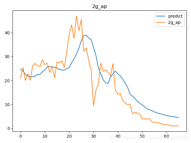
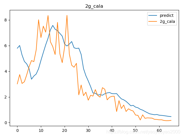
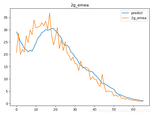
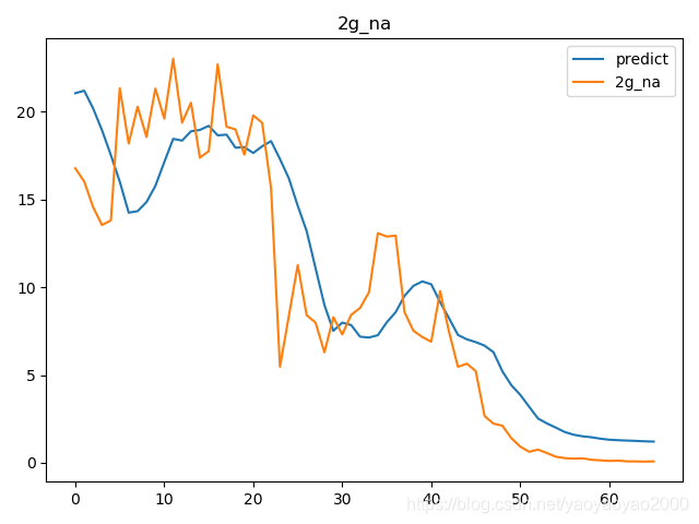
训练结果
预测的数据结果
2020 Q1-Q4 各区域5G规模预测(单位:亿美元)
| 地区\季度 | Q1 | Q2 | Q3 | Q4 |
|---|---|---|---|---|
| AP 5G | 6.890 | 6.717 | 6.581 | 6.493 |
| CALA 5G | 0.819 | 0.634 | 0.474 | 0.369 |
| EMEA 5G | 2.405 | 2.236 | 2.140 | 2.115 |
| NA 5G | 1.899 | 1.766 | 1.562 | 1.694 |
2020 Q1-Q4 各区域无线整体市场规模预测(单位:亿美元)
| 地区\季度 | Q1 | Q2 | Q3 | Q4 |
|---|---|---|---|---|
| AP total | 42.613 | 46.132 | 49.805 | 52.012 |
| CALA total | 6.057 | 6.454 | 6.783 | 6.968 |
| EMEA total | 20.841 | 22.501 | 24.007 | 24.778 |
| NA total | 17.465 | 19.062 | 20.677 | 21.415 |
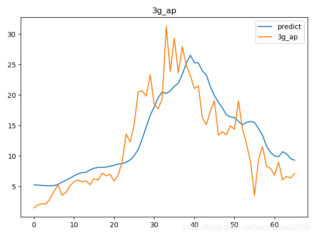
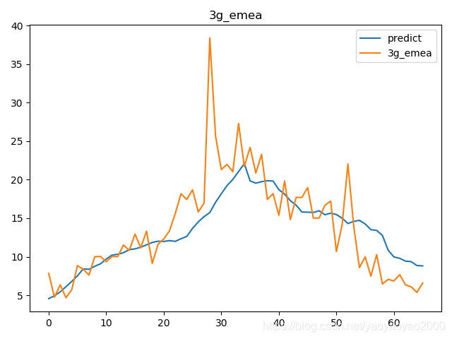
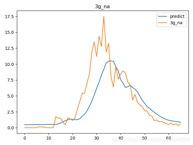
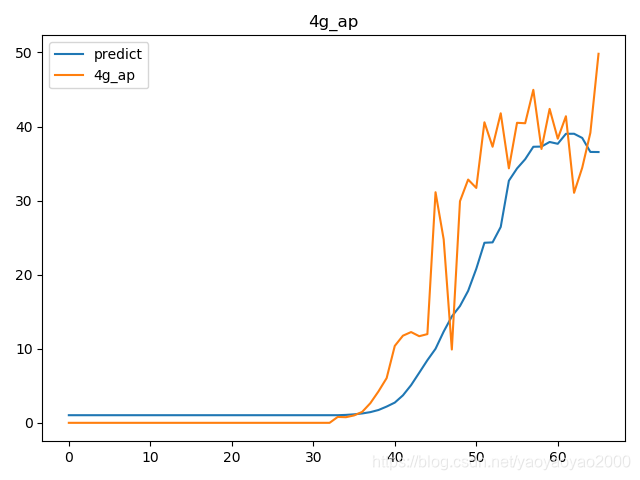
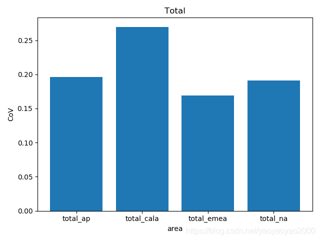
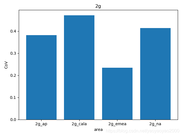
预测结果与实际结果的对比
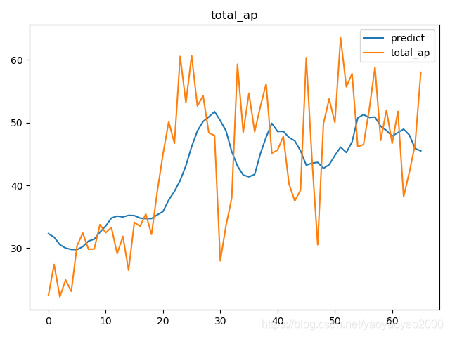
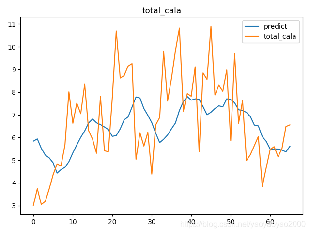
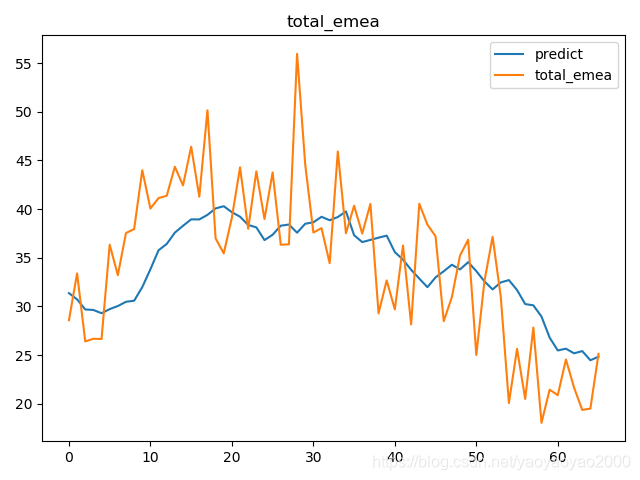
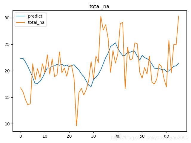

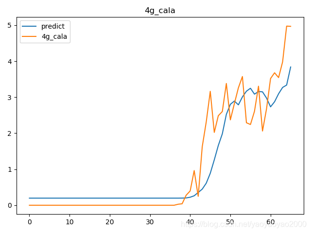

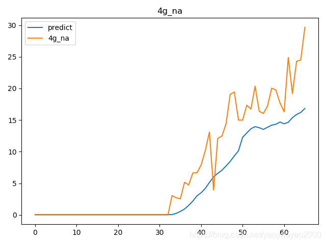
模型评估
我们通过计算每个地区的市场预测结果的变异系数(Coefficient of Variation,CoV)来评估模型预测的准确性。变异系数越高,预测的准确度越差。


完整代码
# importing required libraries
import csv
from typing import List, Anyimport numpy as np
import pandas as pd
from keras.layers import Dense, LSTM
from keras.losses import mean_squared_error
from keras.models import Sequential
from matplotlib import pyplot
from numpy import mean
from sklearn.preprocessing import MinMaxScalerdef total_prediction(file_path, col_g, num):""":param file_path: the path of file read:param col_g: the column we need to read from .csv file:param num: the row number of the .csv file:return: Coefficient of Variation"""# read from csvdf = pd.read_csv(file_path)# sort by row namedata = df.sort_index(ascending=True, axis=0)# creating data framenew_data = pd.DataFrame(index=range(0, len(df)), columns=['Date', col_g])# copy the 'data' read from .csv file to 'new_data'for i in range(0, len(data)):new_data['Date'][i] = data['Date'][i]new_data[col_g][i] = data[col_g][i]# setting index, new_data is the DataFrame type.new_data.index = new_data.Date# drop the 'Date' column of 'new_data'new_data.drop('Date', axis=1, inplace=True)# creating train and test setsdataset = new_data.values# the 0th to num th data was included in train settrain = dataset[0:num-20, :]# the size of test set is 12test_size = 6# to avoid the null prediction, we use the test_size to num of 'dataset' as valid set.valid = dataset[test_size:, :]# converting dataset into x_train and y_train# scaler is used to normalize data within 0 and 1scaler = MinMaxScaler(feature_range=(0, 1))# normalizing datascaled_data = scaler.fit_transform(dataset)x_train, y_train = [], []for i in range(test_size, len(train)):x_train.append(scaled_data[i - test_size:i, 0])y_train.append(scaled_data[i, 0])# convert to numpy# the row of x_train is (num-test_size)=64, the col of x_train is test_size=12# the row of y_train is test_size=12, the col of x_train is 1x_train, y_train = np.array(x_train), np.array(y_train)#  tuple, reshape x_train to be 3D.[samples, timesteps, features], (64,12,1)x_train = np.reshape(x_train, (x_train.shape[0], x_train.shape[1], 1))# create and fit the LSTM network# design networkmodel = Sequential()model.add(LSTM(units=50, return_sequences=True, input_shape=(x_train.shape[1], 1)))model.add(LSTM(units=50))model.add(Dense(1))model.compile(loss='mean_squared_error', optimizer='adam')# fit network# x_train: Input data; y_train: Target data; batch_size:Number of samples per gradient updatehistory = model.fit(x_train, y_train, epochs=3, batch_size=3, verbose=0)# plot loss# pyplot.plot(history.history['loss'], label='train')# pyplot.legend()# pyplot.show()# predicting with past 'test_size' sample from the train data# from len(new_data) - len(valid) - test_size () to endinputs = new_data[len(new_data) - len(valid) - test_size:].values# reshape into one colinputs = inputs.reshape(-1, 1)# Scaling features of inputs according to feature_range.inputs = scaler.transform(inputs)# test the predict result of model, add the data to be predict into x_test listx_test = []# total_size*test_size, 74*6for i in range(test_size, inputs.shape[0]):x_test.append(inputs[i - test_size:i, 0])# convert to numpy arrayx_test = np.array(x_test)# (total_size, test_size, )(74,6,1)x_test = np.reshape(x_test, (x_test.shape[0], x_test.shape[1], 1))# make predictionpredict_result = model.predict(x_test)# inverse the normalized data to originalpredict_result = scaler.inverse_transform(predict_result)# the size of predict_result is num - test_size, the last 4 cannot take into considerationpredict_result = predict_result[0:num - test_size - 4]predict_2020 = predict_result[num - test_size - 4:]valid = valid[:, 0]valid = valid[0:num - test_size - 4]# plot the predict and the actualpyplot.plot(predict_result, label='predict')pyplot.plot(valid, label=col_g)pyplot.title(col_g)pyplot.legend()pyplot.show()print(col_g)# calculate Root Mean Squared Errorrmse = np.sqrt(mean_squared_error(predict_result, valid))# calculate Coefficient of Variationcov = rmse / mean(valid)print('Coefficient of Variation:', rmse / mean(valid))for i in predict_result:float(i)print(i)print("\n")return cov,predict_result,validdef draw_bar(x_index, data_list, xticks, title, x_label, y_label):"""to draw the bar plot:param x_index: index:param data_list: height:param xticks: set the current tick locations labels of the x-axis:param title::param x_label::param y_label::return: null"""pyplot.bar(x_index, data_list)pyplot.xlabel(x_label)pyplot.ylabel(y_label)pyplot.xticks(x_index, xticks)pyplot.title(title)pyplot.show()pyplot.savefig()if __name__ == "__main__":# index = np.arange(4)# cov_rcv = []# print('\nTotal prediction:\n')# cov_rcv.append(total_prediction('AP.csv', 'total_ap', 76))# cov_rcv.append(total_prediction('CALA.csv', 'total_cala', 76))# cov_rcv.append(total_prediction('EMEA.csv', 'total_emea', 76))# cov_rcv.append(total_prediction('NA.csv', 'total_na', 76))# cov_rcv = np.array(cov_rcv)# x_ticks = ('total_ap', 'total_cala', 'total_emea', 'total_na')# draw_bar(index, cov_rcv, x_ticks, 'Total', 'area', 'CoV')predict_result = total_prediction('AP.csv', 'total_ap', 76)[1]valid = total_prediction('AP.csv', 'total_ap', 76)[2]fig = pyplot.figure()ax1 = fig.add_subplot(221)ax1.plot(predict_result, label='predict')ax1.plot(valid, label='total_ap')pyplot.legend()predict_result=total_prediction('CALA.csv', 'total_cala', 76)[1]valid = total_prediction('CALA.csv', 'total_cala', 76)[2]ax2 = fig.add_subplot(222)ax2.plot(predict_result, label='predict')ax2.plot(valid, label='total_cala')pyplot.legend()predict_result=total_prediction('EMEA.csv', 'total_emea', 76)[1]valid = total_prediction('EMEA.csv', 'total_emea', 76)[2]ax3 = fig.add_subplot(223)ax3.plot(predict_result, label='predict')ax3.plot(valid, label='total_emea')pyplot.legend()predict_result=total_prediction('NA.csv', 'total_na', 76)[1]valid = total_prediction('NA.csv', 'total_na', 76)[2]ax4 = fig.add_subplot(224)ax4.plot(predict_result, label='predict')ax4.plot(valid, label='total_na')pyplot.legend()pyplot.show()# print('\n2g prediction:\n')# cov_2g = [total_prediction('AP.csv', '2g_ap', 76), total_prediction('CALA.csv', '2g_cala', 76),#           total_prediction('EMEA.csv', '2g_emea', 76), total_prediction('NA.csv', '2g_na', 76)]# cov_2g = np.array(cov_2g)# x_ticks = ('2g_ap', '2g_cala', '2g_emea', '2g_na')# draw_bar(index, cov_2g, x_ticks, '2g', 'area', 'CoV')## print('\n3g prediction:\n')# cov_3g = [total_prediction('AP.csv', '3g_ap', 76), total_prediction('CALA.csv', '3g_cala', 76),#           total_prediction('EMEA.csv', '3g_emea', 76), total_prediction('NA.csv', '3g_na', 76)]# cov_3g = np.array(cov_3g)# x_ticks = ('3g_ap', '3g_cala', '3g_emea', '3g_na')# draw_bar(index, cov_3g, x_ticks, '3g', 'area', 'CoV')## print('\n4g prediction:\n')# cov_4g = [total_prediction('AP.csv', '4g_ap', 76), total_prediction('CALA.csv', '4g_cala', 76),#           total_prediction('EMEA.csv', '4g_emea', 76), total_prediction('NA.csv', '4g_na', 76)]# cov_4g = np.array(cov_4g)# x_ticks = ('4g_ap', '4g_cala', '4g_emea', '4g_na')# draw_bar(index, cov_4g, x_ticks, '4g', 'area', 'CoV')# total_prediction('AP.csv', '2g_ap', 76)# total_prediction('CALA.csv', '2g_cala', 76)# total_prediction('EMEA.csv', '2g_emea', 76)# total_prediction('NA.csv', '2g_na', 76)## total_prediction('AP.csv', '3g_ap', 76)# total_prediction('CALA.csv', '3g_cala', 76)# total_prediction('EMEA.csv', '3g_emea', 76)# total_prediction('NA.csv', '3g_na', 76)## total_prediction('AP.csv', '4g_ap', 76)# total_prediction('CALA.csv', '4g_cala', 76)# total_prediction('EMEA.csv', '4g_emea', 76)# total_prediction('NA.csv', '4g_na', 76)
参考链接
https://blog.csdn.net/qq_28031525/article/details/79046718
本文来自互联网用户投稿,文章观点仅代表作者本人,不代表本站立场,不承担相关法律责任。如若转载,请注明出处。 如若内容造成侵权/违法违规/事实不符,请点击【内容举报】进行投诉反馈!