彻底搞懂NeRF论文公式代码

这周一直在死磕nerf，做个总结，代码主要是基于Nerf-pytorch，我愿称之为最好部署的nerf

GitHub - yenchenlin/nerf-pytorch: A PyTorch implementation of NeRF (Neural Radiance Fields) that reproduces the results.

NeRF工作的过程可以分成两部分：三维重建和渲染。

三维重建部分本质上是一个2D到3D的建模过程，利用3D点的位置（x，y，z）及方位视角（θ，φ）作为输入，通过多层感知机（MLP）建模该点对应的颜色color（c）及体素密度volume density（σ），形成了3D场景的”隐式表示“。

此处2D的输入包括 'llff'、'blender'、'LINEMOD'、'deepvoxels' 四种类型的数据集。其中的llff如前文所讲，是经过colmap处理之后N张图片形成的N*17矩阵，也就是论文中讲的5D输入（不同的数据集可能有不同的输入？没有全部仔细看过）。

具体而言读取数据集返回为

images, poses, render_poses, hwf, i_split = load_blender_data(args.datadir, args.half_res, args.testskip)

basedir是基路径，half_res默认为False，同时lego数据集中的默认训练图片规格为 800×800 ，当该参数为True，则需要将图片规格转化为 400×400；

testskip的值为N，则会从测试集和验证集中挑选 1/N数量作为测试集和验证集，相当于跳跃步长。

接着这里将训练、验证、测试数据对应的json文件都读入进来，并用一个名为metas的字典存储。这些json文件中存储的都是图片对应的相机参数以及外参矩阵信息等。焦距图像来自于大佬的博客

NeRF Pytorch 代码笔记_nerf代码_威尔士矮脚狗的博客-CSDN博客

 

pose_spherical函数的计算过程可以参考下图

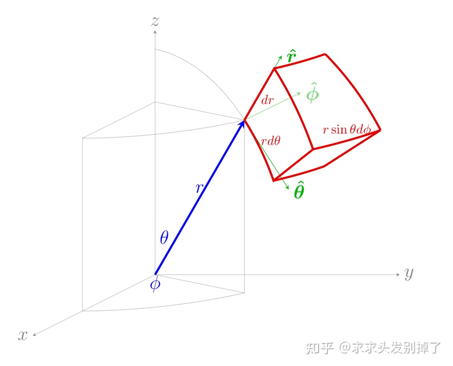
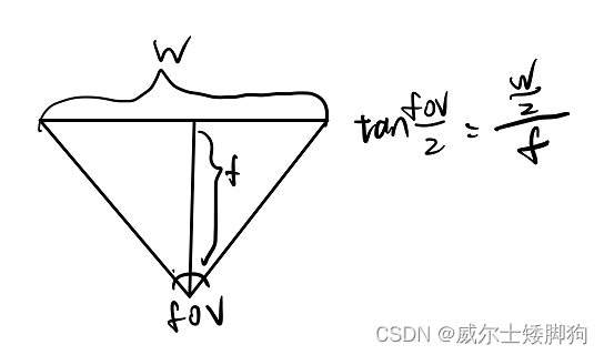
def load_blender_data(basedir, half_res=False, testskip=1)://读取三个文件夹中的图像和transforms.json里的信息splits = ['train', 'val', 'test']metas = {}for s in splits:with open(os.path.join(basedir, 'transforms_{}.json'.format(s)), 'r') as fp://meta：'camera_angle_x'相机的水平视场 (horizontal field of view)，可以用于算焦距 (focal)，'frames'里面有图片路径、图片的相机外参transform_matrix和旋转值rotation(未用到)metas[s] = json.load(fp)//获取img及相机外参posesall_imgs = []all_poses = []counts = [0]for s in splits:meta = metas[s]imgs = []poses = []//testskip相当于跳跃选择图像，在测试时减少计算量if s=='train' or testskip==0:skip = 1else:skip = testskipfor frame in meta['frames'][::skip]:fname = os.path.join(basedir, frame['file_path'] + '.png')imgs.append(imageio.imread(fname))poses.append(np.array(frame['transform_matrix']))//list变成np[100,800,800,4],除255实现图像归一化imgs = (np.array(imgs) / 255.).astype(np.float32) # keep all 4 channels (RGBA)poses = np.array(poses).astype(np.float32)counts.append(counts[-1] + imgs.shape[0])all_imgs.append(imgs)all_poses.append(poses)//count最后结果是[0,i_train,i_train+i_val,i_train+i_val+i_test]//i_split就是将三个数据划分开i_split = [np.arange(counts[i], counts[i+1]) for i in range(3)]//imgs和poses目前是根据三个集划分的list，在0维拼接，最后变成[i_train+i_val+i_test,800,800,4]和[i_train+i_val+i_test,4,4]imgs = np.concatenate(all_imgs, 0)poses = np.concatenate(all_poses, 0)//图像的高宽以及相机视角，focal计算公式tan(fov/2)=w/2/f,fov即相机的水平视场H, W = imgs[0].shape[:2]camera_angle_x = float(meta['camera_angle_x'])focal = .5 * W / np.tan(.5 * camera_angle_x)//其中np.linspace(-180,180,40+1)生成了一个范围从-180到180，相邻间隔为180-（-180）/40=9的，元素数量为40+1=41的一维数组。而后续的[:-1]则抛弃了最后一个元素，最终结果为[-180,-171,...,171]。render_poses = torch.stack([pose_spherical(angle, -30.0, 4.0) for angle in np.linspace(-180,180,40+1)[:-1]], 0)//pose_spherical的代码如下，输入phi为方位角，theta为仰角，radius为距离球心距离，其中phi和radius默认为-30和4，angle则是[-180,-171,...,171]
//这一整个过程即根据公式计算c2w矩阵，render_poses最终产生40个[4,4]的变换矩阵，这其实是40个相机位姿，即用来生成一个相机轨迹用于新视角的合成
def pose_spherical(theta, phi, radius):c2w = trans_t(radius)c2w = rot_phi(phi/180.*np.pi) @ c2wc2w = rot_theta(theta/180.*np.pi) @ c2wc2w = torch.Tensor(np.array([[-1,0,0,0],[0,0,1,0],[0,1,0,0],[0,0,0,1]])) @ c2wreturn c2wtrans_t = lambda t : torch.Tensor([[1,0,0,0],[0,1,0,0],[0,0,1,t],[0,0,0,1]]).float()rot_phi = lambda phi : torch.Tensor([[1,0,0,0],[0,np.cos(phi),-np.sin(phi),0],[0,np.sin(phi), np.cos(phi),0],[0,0,0,1]]).float()rot_theta = lambda th : torch.Tensor([[np.cos(th),0,-np.sin(th),0],[0,1,0,0],[np.sin(th),0, np.cos(th),0],[0,0,0,1]]).float()
////用插值法生成一半大小的图像，减少内存占用，同时焦距也减半if half_res:H = H//2W = W//2focal = focal/2.imgs_half_res = np.zeros((imgs.shape[0], H, W, 4))for i, img in enumerate(imgs):imgs_half_res[i] = cv2.resize(img, (W, H), interpolation=cv2.INTER_AREA)imgs = imgs_half_res# imgs = tf.image.resize_area(imgs, [400, 400]).numpy()return imgs, poses, render_poses, [H, W, focal], i_split

image N*H*W*4，pose N*4*4，render_pose 40*4*4，hwf 是最后一列的HWF，i_split是训练集、测试集、验证集的划分情况

image为RGBA，A为alpha，意为不透明度

这里的pose是4*4，实际上是3*4的矩阵，最后一行是0，0，0，1，和前文的变换矩阵的前4列一致。

render_pose和pose一样，实际上是3*4的矩阵，是相机轨迹用于新视角的合成，这里先不展开讲了。

接下来blender数据集是指定了near和far，而在其他数据集格式了这两个值是可以被计算的

        near = 2.far = 6.if args.white_bkgd:images = images[...,:3]*images[...,-1:] + (1.-images[...,-1:])else:images = images[...,:3]

white_bkgd消除掉了RGBA的A，并且将渲染背景定位白色？

将H,W修正为整数，并设置相机内参K

    # Cast intrinsics to right typesH, W, focal = hwfH, W = int(H), int(W)hwf = [H, W, focal]if K is None:K = np.array([[focal, 0, 0.5*W],[0, focal, 0.5*H],[0, 0, 1]])

接着就到了创建模型，创建模型这里细讲，
render_kwargs_train, render_kwargs_test, start, grad_vars, optimizer = create_nerf(args)

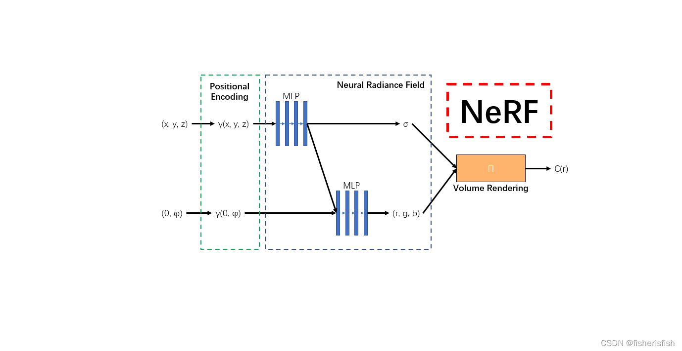NeRF模型的作用通过多层感知机（MLP）建模该点对应的颜色color（c）及体素密度volume density（σ），形成了3D场景的”隐式表示“，那么具体做法如上图，图中的Positional encoding是作者发现让①中的MLP网络(F：(x，d) -> (c，σ))直接操作 (x，y，z，θ，φ)输入会导致渲染在表示颜色和几何形状方面的高频变化方面表现不佳，表明深度网络偏向于学习低频函数。因此在将(x，y，z，θ，φ)输入传递给网络之前，使用高频函数将输入映射到更高维度的空间，可以更好地拟合包含高频变化的数据。

 在模型的开头，就调用了一个编码函数，这个函数是给xyz位置编码的，输入是multires和i_embed，前者是10，就是映射的高维数，后者是0，用来判断是否需要编码，此函数返回一个编码器embed_fn以及编码后的维数out_dim，以xyz位置编码为例，out_dim=10(multires)*2(cos、sin)*3(xyz)+3(xyz)=63,其中编码器可以理解为一个返回值为编码后向量的函数。对应的即为论文中的位置编码。

embed_fn, input_ch = get_embedder(args.multires, args.i_embed)def get_embedder(multires, i=0):if i == -1:return nn.Identity(), 3embed_kwargs = {'include_input' : True,'input_dims' : 3,'max_freq_log2' : multires-1,'num_freqs' : multires,'log_sampling' : True,'periodic_fns' : [torch.sin, torch.cos],}embedder_obj = Embedder(**embed_kwargs)embed = lambda x, eo=embedder_obj : eo.embed(x)return embed, embedder_obj.out_dim# Positional encoding (section 5.1)
class Embedder:def __init__(self, **kwargs):self.kwargs = kwargsself.create_embedding_fn()def create_embedding_fn(self):embed_fns = []d = self.kwargs['input_dims']out_dim = 0if self.kwargs['include_input']:embed_fns.append(lambda x : x)out_dim += dmax_freq = self.kwargs['max_freq_log2']N_freqs = self.kwargs['num_freqs']if self.kwargs['log_sampling']:freq_bands = 2.**torch.linspace(0., max_freq, steps=N_freqs)else:freq_bands = torch.linspace(2.**0., 2.**max_freq, steps=N_freqs)for freq in freq_bands:for p_fn in self.kwargs['periodic_fns']:embed_fns.append(lambda x, p_fn=p_fn, freq=freq : p_fn(x * freq))out_dim += dself.embed_fns = embed_fnsself.out_dim = out_dimdef embed(self, inputs):return torch.cat([fn(inputs) for fn in self.embed_fns], -1)

 这一段就是对θ，φ编码的编码器函数，以及模型输入，netdepth论文里提到了是8，8层MLP，netwidth是256，inputch是63，outputch是5，skips为4，但不清楚具体作用，后文再看，args.use_viewdirs为True表示输入包含方向信息，以5D的向量作为输入，否则仅由位置信息作为3D输入。这里的N_importance即为论文中在粗网络之后采样的 Nf个基于粗网络分布的点。粗网络来自于Hierarchical volume sampling方法，

该部分指出在Volume Rendering中是在每条相机光线上的N个查询点密集地评估神经辐射场网络，这是低效的（仍然重复采样与渲染图像无关的自由空间和遮挡区域），于是提出一种分层体积采样的做法，同时优化一个“粗糙”的网络和一个“精细”的网络。

做法是：首先使用分层抽样对第一组Nc位置进行采样，并在这些位置评估“粗糙”网络。给出这个“粗糙”网络的输出，然后我们对每条射线上的点进行更明智的采样，即利用反变换采样从这个分布中采样第二组Nf位置，然后将Nc+Nf采样得到的数据输入“精细”网络，并计算最终渲染的光线颜色C(r)。具体实现方法后面再看。

    input_ch_views = 0embeddirs_fn = Noneif args.use_viewdirs:embeddirs_fn, input_ch_views = get_embedder(args.multires_views, args.i_embed)output_ch = 5 if args.N_importance > 0 else 4skips = [4]model = NeRF(D=args.netdepth, W=args.netwidth,input_ch=input_ch, output_ch=output_ch, skips=skips,input_ch_views=input_ch_views, use_viewdirs=args.use_viewdirs).to(device)

 pts_linears8层MLP,skips控制在第五层输入变成了319，结合模型图可以看懂是什么意思，插入了方位视角（θ，φ）的信息，skips控制插入的层数，实际上这里结合的是xyz本身的输入，是一个跳跃连接，319=256+63，上面的图有一定的错误，实际模型可以参考这幅图

ModuleList((0): Linear(in_features=63, out_features=256, bias=True)(1): Linear(in_features=256, out_features=256, bias=True)(2): Linear(in_features=256, out_features=256, bias=True)(3): Linear(in_features=256, out_features=256, bias=True)(4): Linear(in_features=256, out_features=256, bias=True)(5): Linear(in_features=319, out_features=256, bias=True)(6): Linear(in_features=256, out_features=256, bias=True)(7): Linear(in_features=256, out_features=256, bias=True)
)

class NeRF(nn.Module):def __init__(self, D=8, W=256, input_ch=3, input_ch_views=3, output_ch=4, skips=[4], use_viewdirs=False):""" """super(NeRF, self).__init__()self.D = Dself.W = Wself.input_ch = input_chself.input_ch_views = input_ch_viewsself.skips = skipsself.use_viewdirs = use_viewdirsself.pts_linears = nn.ModuleList([nn.Linear(input_ch, W)] + [nn.Linear(W, W) if i not in self.skips else nn.Linear(W + input_ch, W) for i in range(D-1)])### Implementation according to the official code release (https://github.com/bmild/nerf/blob/master/run_nerf_helpers.py#L104-L105)self.views_linears = nn.ModuleList([nn.Linear(input_ch_views + W, W//2)])### Implementation according to the paper# self.views_linears = nn.ModuleList(#     [nn.Linear(input_ch_views + W, W//2)] + [nn.Linear(W//2, W//2) for i in range(D//2)])if use_viewdirs:self.feature_linear = nn.Linear(W, W)self.alpha_linear = nn.Linear(W, 1)self.rgb_linear = nn.Linear(W//2, 3)else:self.output_linear = nn.Linear(W, output_ch)

前向推理部分，我们后续得到了输入再讲，在下一步中定义了细网络，lego.txt中给出N_importance是128，即对应 Nf=128 。和之前的网络相比，参数均没有变化

    grad_vars = list(model.parameters())model_fine = Noneif args.N_importance > 0:model_fine = NeRF(D=args.netdepth_fine, W=args.netwidth_fine,input_ch=input_ch, output_ch=output_ch, skips=skips,input_ch_views=input_ch_views, use_viewdirs=args.use_viewdirs).to(device)grad_vars += list(model_fine.parameters())

这里调用了run_network()函数。 

    network_query_fn = lambda inputs, viewdirs, network_fn : run_network(inputs, viewdirs, network_fn,embed_fn=embed_fn,embeddirs_fn=embeddirs_fn,netchunk=args.netchunk)

先看函数头，inputs为输入；viewdirs为方向信息；fn为网络；embed_fn为位置编码器；embeddirs_fn为方向编码器；netchunk为并行处理的点的数量。 

先将输入展平为向量，随后进行位置信息编码。如果采用方向信息，则对方向信息进行编码并和位置信息的编码合并。使用batchify函数进行批处理，fn为采用的网络，netchunk为并行处理的输入数量，embedded为编码后的输入点。随后对展平的输出重新恢复形状后返回。总结就是输入到输出的过程。

def run_network(inputs, viewdirs, fn, embed_fn, embeddirs_fn, netchunk=1024*64):"""Prepares inputs and applies network 'fn'."""inputs_flat = torch.reshape(inputs, [-1, inputs.shape[-1]])embedded = embed_fn(inputs_flat)if viewdirs is not None:input_dirs = viewdirs[:,None].expand(inputs.shape)input_dirs_flat = torch.reshape(input_dirs, [-1, input_dirs.shape[-1]])embedded_dirs = embeddirs_fn(input_dirs_flat)embedded = torch.cat([embedded, embedded_dirs], -1)outputs_flat = batchify(fn, netchunk)(embedded)outputs = torch.reshape(outputs_flat, list(inputs.shape[:-1]) + [outputs_flat.shape[-1]])return outputs

 定义优化器

    optimizer = torch.optim.Adam(params=grad_vars, lr=args.lrate, betas=(0.9, 0.999))start = 0basedir = args.basedirexpname = args.expname

 加载预训练权重

    # Load checkpointsif args.ft_path is not None and args.ft_path!='None':ckpts = [args.ft_path]else:ckpts = [os.path.join(basedir, expname, f) for f in sorted(os.listdir(os.path.join(basedir, expname))) if 'tar' in f]print('Found ckpts', ckpts)if len(ckpts) > 0 and not args.no_reload:ckpt_path = ckpts[-1]print('Reloading from', ckpt_path)ckpt = torch.load(ckpt_path)start = ckpt['global_step']optimizer.load_state_dict(ckpt['optimizer_state_dict'])# Load modelmodel.load_state_dict(ckpt['network_fn_state_dict'])if model_fine is not None:model_fine.load_state_dict(ckpt['network_fine_state_dict'])

 对返回值进行处理

render_kwargs_train = {'network_query_fn' : network_query_fn,#匿名函数，给定三位点、方向，利用给定网络求解RGBA'perturb' : args.perturb,'N_importance' : args.N_importance,#每条光线上细采样点的数量'network_fine' : model_fine,#精细网络'N_samples' : args.N_samples,#每条光线上粗采样点的数量'network_fn' : model,#粗网络'use_viewdirs' : args.use_viewdirs,#是否使用视点方向'white_bkgd' : args.white_bkgd,#是否将透明背景用白色填充'raw_noise_std' : args.raw_noise_std,#归一化密度
}# NDC only good for LLFF-style forward facing data
if args.dataset_type != 'llff' or args.no_ndc:print('Not ndc!')render_kwargs_train['ndc'] = Falserender_kwargs_train['lindisp'] = args.lindisprender_kwargs_test = {k : render_kwargs_train[k] for k in render_kwargs_train}
render_kwargs_test['perturb'] = False
render_kwargs_test['raw_noise_std'] = 0.return render_kwargs_train, render_kwargs_test, start, grad_vars, optimizer

 train和test基本上是一致的，start是开始时的epoch数，不加载预训练权重是为0，grad_vars和optimizer是反向梯度传播和优化器

{'network_query_fn': . at 0x000002838FAF99D8>, 'perturb': 1.0, 'N_importance': 128, 'network_fine': NeRF((pts_linears): ModuleList((0): Linear(in_features=63, out_features=256, bias=True)(1): Linear(in_features=256, out_features=256, bias=True)(2): Linear(in_features=256, out_features=256, bias=True)(3): Linear(in_features=256, out_features=256, bias=True)(4): Linear(in_features=256, out_features=256, bias=True)(5): Linear(in_features=319, out_features=256, bias=True)(6): Linear(in_features=256, out_features=256, bias=True)(7): Linear(in_features=256, out_features=256, bias=True))(views_linears): ModuleList((0): Linear(in_features=283, out_features=128, bias=True))(feature_linear): Linear(in_features=256, out_features=256, bias=True)(alpha_linear): Linear(in_features=256, out_features=1, bias=True)(rgb_linear): Linear(in_features=128, out_features=3, bias=True)
), 'N_samples': 64, 'network_fn': NeRF((pts_linears): ModuleList((0): Linear(in_features=63, out_features=256, bias=True)(1): Linear(in_features=256, out_features=256, bias=True)(2): Linear(in_features=256, out_features=256, bias=True)(3): Linear(in_features=256, out_features=256, bias=True)(4): Linear(in_features=256, out_features=256, bias=True)(5): Linear(in_features=319, out_features=256, bias=True)(6): Linear(in_features=256, out_features=256, bias=True)(7): Linear(in_features=256, out_features=256, bias=True))(views_linears): ModuleList((0): Linear(in_features=283, out_features=128, bias=True))(feature_linear): Linear(in_features=256, out_features=256, bias=True)(alpha_linear): Linear(in_features=256, out_features=1, bias=True)(rgb_linear): Linear(in_features=128, out_features=3, bias=True)
), 'use_viewdirs': True, 'white_bkgd': True, 'raw_noise_std': 0.0, 'ndc': False, 'lindisp': False}

模型初始化之后返回train函数，给render_kwargs_train加上了near和far

    global_step = startbds_dict = {'near' : near,'far' : far,}render_kwargs_train.update(bds_dict)render_kwargs_test.update(bds_dict)# Move testing data to GPUrender_poses = torch.Tensor(render_poses).to(device)

 仅运行渲染视频

    # Short circuit if only rendering out from trained modelif args.render_only:print('RENDER ONLY')with torch.no_grad():if args.render_test:# render_test switches to test posesimages = images[i_test]else:# Default is smoother render_poses pathimages = Nonetestsavedir = os.path.join(basedir, expname, 'renderonly_{}_{:06d}'.format('test' if args.render_test else 'path', start))os.makedirs(testsavedir, exist_ok=True)print('test poses shape', render_poses.shape)rgbs, _ = render_path(render_poses, hwf, K, args.chunk, render_kwargs_test, gt_imgs=images, savedir=testsavedir, render_factor=args.render_factor)print('Done rendering', testsavedir)imageio.mimwrite(os.path.join(testsavedir, 'video.mp4'), to8b(rgbs), fps=30, quality=8)return

use_batching = not args.no_batching从多张图中取用光线，特别的，对于lego数据集来说，并没有采用该策略。所以这段代码在lego重建过程中，是不运行的，这里我们先跳过，当中的核心函数过程为get_rays_np()。

    # Prepare raybatch tensor if batching random raysN_rand = args.N_randuse_batching = not args.no_batchingif use_batching:# For random ray batchingprint('get rays')rays = np.stack([get_rays_np(H, W, K, p) for p in poses[:,:3,:4]], 0) # [N, ro+rd, H, W, 3]print('done, concats')rays_rgb = np.concatenate([rays, images[:,None]], 1) # [N, ro+rd+rgb, H, W, 3]rays_rgb = np.transpose(rays_rgb, [0,2,3,1,4]) # [N, H, W, ro+rd+rgb, 3]rays_rgb = np.stack([rays_rgb[i] for i in i_train], 0) # train images onlyrays_rgb = np.reshape(rays_rgb, [-1,3,3]) # [(N-1)*H*W, ro+rd+rgb, 3]rays_rgb = rays_rgb.astype(np.float32)print('shuffle rays')np.random.shuffle(rays_rgb)print('done')i_batch = 0# Move training data to GPUif use_batching:images = torch.Tensor(images).to(device)poses = torch.Tensor(poses).to(device)if use_batching:rays_rgb = torch.Tensor(rays_rgb).to(device)

设置训练的iters，打印训练集、测试集、验证集信息

    N_iters = 200000 + 1print('Begin')print('TRAIN views are', i_train)print('TEST views are', i_test)print('VAL views are', i_val)TRAIN views are [ 0  1  2  3  4  5  6  7  8  9 10 11 12 13 14 15 16 17 18 19 20 21 22 2324 25 26 27 28 29 30 31 32 33 34 35 36 37 38 39 40 41 42 43 44 45 46 4748 49 50 51 52 53 54 55 56 57 58 59 60 61 62 63 64 65 66 67 68 69 70 7172 73 74 75 76 77 78 79 80 81 82 83 84 85 86 87 88 89 90 91 92 93 94 9596 97 98 99]
TEST views are [113 114 115 116 117 118 119 120 121 122 123 124 125 126 127 128 129 130131 132 133 134 135 136 137]
VAL views are [100 101 102 103 104 105 106 107 108 109 110 111 112]

 开始迭代，这一段不运行，我们直接看else后面的内容

    start = start + 1for i in trange(start, N_iters):time0 = time.time()# Sample random ray batchif use_batching:# Random over all imagesbatch = rays_rgb[i_batch:i_batch+N_rand] # [B, 2+1, 3*?]batch = torch.transpose(batch, 0, 1)batch_rays, target_s = batch[:2], batch[2]i_batch += N_randif i_batch >= rays_rgb.shape[0]:print("Shuffle data after an epoch!")rand_idx = torch.randperm(rays_rgb.shape[0])rays_rgb = rays_rgb[rand_idx]i_batch = 0

else开始的部分是读取单张图片，这里pose就是只读取了N*3*4的有效信息 

 else:# Random from one imageimg_i = np.random.choice(i_train)target = images[img_i]target = torch.Tensor(target).to(device)pose = poses[img_i, :3,:4]

get_rays是run_nerf_helpers里面定义的函数，其和之前的get_rays_np作用类似，从单张图中取用光线，

先在三维空间利用几何关系和内参矩阵K求得表示光线方向的向量；

随后利用外参矩阵将相机坐标系变换到世界坐标系；

H，W是输入图像的高宽，K是相机内参，由之前定义,c2w就是之前提到的相机变换至世界坐标系，也就是pose。

if N_rand is not None:rays_o, rays_d = get_rays(H, W, K, torch.Tensor(pose))  # (H, W, 3), (H, W, 3)# Ray helpers
def get_rays(H, W, K, c2w):i, j = torch.meshgrid(torch.linspace(0, W-1, W), torch.linspace(0, H-1, H))  # pytorch's meshgrid has indexing='ij'i = i.t()j = j.t()dirs = torch.stack([(i-K[0][2])/K[0][0], -(j-K[1][2])/K[1][1], -torch.ones_like(i)], -1)# Rotate ray directions from camera frame to the world framerays_d = torch.sum(dirs[..., np.newaxis, :] * c2w[:3,:3], -1)  # dot product, equals to: [c2w.dot(dir) for dir in dirs]# Translate camera frame's origin to the world frame. It is the origin of all rays.rays_o = c2w[:3,-1].expand(rays_d.shape)return rays_o, rays_dif K is None:K = np.array([[focal, 0, 0.5*W],[0, focal, 0.5*H],[0, 0, 1]])

i, j = torch.meshgrid(torch.linspace(0, W-1, W), torch.linspace(0, H-1, H))生成坐标

 torch.meshgrid（）的功能是生成网格，可以用于生成坐标。函数输入两个数据类型相同的一维张量，两个输出张量的行数为第一个输入张量的元素个数，列数为第二个输入张量的元素个数，当两个输入张量数据类型不同或维度不是一维时会报错。

torch.linspace(start, end, steps=100, out=None, dtype=None, layout=torch.strided, device=None, requires_grad=False) → Tensor
函数的作用是，返回一个一维的tensor（张量），这个张量包含了从start到end（包括端点）的等距的steps个数据点。

 torch.t()是一个类似于求矩阵的转置的函数，但是它要求输入的tensor结构维度<=2D。 这里参考大佬的博客。

(62条消息) 线性代数：转置矩阵（matrix transpose）和逆矩阵（matrix inverse）_逆矩阵和转置矩阵_羊羊2035的博客-CSDN博客

i = i.t()
j = j.t()

接下来这个公式解读可以参考大佬的知乎里的3D空间射线怎么构造章节

NeRF代码解读-相机参数与坐标系变换 - 知乎 (zhihu.com)

最后我们看一下这个射线是怎么构造的。给定一张图像的一个像素点，我们的目标是构造以相机中心为起始点，经过相机中心和像素点的射线。

首先，明确两件事：

1. 一条射线包括一个起始点和一个方向，起点的话就是相机中心。对于射线方向，我们都知道两点确定一条直线，所以除了相机中心我们还需另一个点，而这个点就是成像平面的像素点。
2. NeRF代码是在相机坐标系下构建射线，然后再通过camera-to-world (c2w)矩阵将射线变换到世界坐标系。

通过上述的讨论，我们第一步是要先写出相机中心和像素点在相机坐标系的3D坐标。下面我们以OpenCV/Colmap的相机坐标系为例介绍。相机中心的坐标很明显就是[0,0,0]了。像素点的坐标可能复杂一点：首先3D像素点的x和y坐标是2D的图像坐标 (i, j)减去光心坐标 (cx,cy)，然后z坐标其实就是焦距f (因为图像平面距离相机中心的距离就是焦距f)。

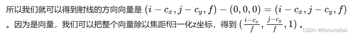
dirs = torch.stack([(i-K[0][2])/K[0][0], -(j-K[1][2])/K[1][1], -torch.ones_like(i)], -1)

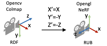
所以K[0][0]和K[1][1]就是focal，也就是焦距，K[0][2]是Cx，也就是W/2，K[1][2]是Cy，也就是H/2，公式里的负号是因为OpenCV/Colmap的相机坐标系里相机的Up/Y朝下, 相机光心朝向+Z轴，而NeRF/OpenGL相机坐标系里相机的Up/朝上，相机光心朝向-Z轴，所以这里代码在方向向量dir的第二和第三项乘了个负号。

 这是得到dirs的值，torch.stack将其叠成了一个400*400*3的矩阵

tensor([[[-0.3600,  0.3600, -1.0000],[-0.3582,  0.3600, -1.0000],[-0.3564,  0.3600, -1.0000],...,[ 0.3546,  0.3600, -1.0000],[ 0.3564,  0.3600, -1.0000],[ 0.3582,  0.3600, -1.0000]],[[-0.3600,  0.3582, -1.0000],[-0.3582,  0.3582, -1.0000],[-0.3564,  0.3582, -1.0000],...,[ 0.3546,  0.3582, -1.0000],[ 0.3564,  0.3582, -1.0000],[ 0.3582,  0.3582, -1.0000]],[[-0.3600,  0.3564, -1.0000],[-0.3582,  0.3564, -1.0000],[-0.3564,  0.3564, -1.0000],...,[ 0.3546,  0.3564, -1.0000],[ 0.3564,  0.3564, -1.0000],[ 0.3582,  0.3564, -1.0000]],...,[[-0.3600, -0.3546, -1.0000],[-0.3582, -0.3546, -1.0000],[-0.3564, -0.3546, -1.0000],...,[ 0.3546, -0.3546, -1.0000],[ 0.3564, -0.3546, -1.0000],[ 0.3582, -0.3546, -1.0000]],[[-0.3600, -0.3564, -1.0000],[-0.3582, -0.3564, -1.0000],[-0.3564, -0.3564, -1.0000],...,[ 0.3546, -0.3564, -1.0000],[ 0.3564, -0.3564, -1.0000],[ 0.3582, -0.3564, -1.0000]],[[-0.3600, -0.3582, -1.0000],[-0.3582, -0.3582, -1.0000],[-0.3564, -0.3582, -1.0000],...,[ 0.3546, -0.3582, -1.0000],[ 0.3564, -0.3582, -1.0000],[ 0.3582, -0.3582, -1.0000]]])

# Rotate ray directions from camera frame to the world frame
rays_d = torch.sum(dirs[..., np.newaxis, :] * c2w[:3,:3], -1)  # dot product, equals to: [c2w.dot(dir) for dir in dirs]

１．torch.sum(input, dtype=None)
２．torch.sum(input, list: dim, bool: keepdim=False, dtype=None) → Tensorinput:输入一个tensor
dim:要求和的维度，可以是一个列表
keepdim:求和之后这个dim的元素个数为１，所以要被去掉，如果要保留这个维度，则应当keepdim=True

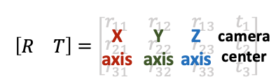
dirs[...,np.newaxis,:]这个操作给dirs新加了一个维度，变成了400*400*1*3，这是基于numpy的广播机制，可以知道，它这里插入一个新的1维度，可以让逐点乘法*得以完成。c2w[:3,:3] 即3列分别表达关于x轴、y轴、z轴的信息，乘完以后变成400*400*3*3，torch.sum对3*3的列求和，就变成了3*1，这和坐标变换公式是一致，只能说非常巧妙了。我的理解是这个计算将相机坐标系下的3D空间射线方向矩阵，转换到世界坐标系下。最终的rays_d就是400*400*3，3是射线在世界坐标系下的射线方向

dot product, equals to: [c2w.dot(dir) for dir in dirs]

即每个dir是锁定了横坐标的点坐标数据，然后被c2w左乘。

(65条消息) numpy广播机制_红烧code的博客-CSDN博客

# Translate camera frame's origin to the world frame. It is the origin of all rays.
rays_o = c2w[:3,-1].expand(rays_d.shape)

c2w[:3,-1]获取转换矩阵最后一列的旋转矩阵，其实就是相机中心点的世界坐标，expand(rays_d.shape)复制成400*400*3，最后返回

rays_o, rays_d，rays_o即射线的原点，rays_d是射线的方向，总共有400*400个像素点，就有400*400个射线。

 返回之后的后续操作

                if i < args.precrop_iters:dH = int(H//2 * args.precrop_frac)dW = int(W//2 * args.precrop_frac)coords = torch.stack(torch.meshgrid(torch.linspace(H//2 - dH, H//2 + dH - 1, 2*dH), torch.linspace(W//2 - dW, W//2 + dW - 1, 2*dW)), -1)if i == start:print(f"[Config] Center cropping of size {2*dH} x {2*dW} is enabled until iter {args.precrop_iters}")                else:coords = torch.stack(torch.meshgrid(torch.linspace(0, H-1, H), torch.linspace(0, W-1, W)), -1)  # (H, W, 2)coords = torch.reshape(coords, [-1,2])  # (H * W, 2)select_inds = np.random.choice(coords.shape[0], size=[N_rand], replace=False)  # (N_rand,)select_coords = coords[select_inds].long()  # (N_rand, 2)rays_o = rays_o[select_coords[:, 0], select_coords[:, 1]]  # (N_rand, 3)rays_d = rays_d[select_coords[:, 0], select_coords[:, 1]]  # (N_rand, 3)batch_rays = torch.stack([rays_o, rays_d], 0)target_s = target[select_coords[:, 0], select_coords[:, 1]]  # (N_rand, 3)

 这一段内容是为了得到一个coords，precrop_iters、frac是configs给出的，意思是对图像中更中心的区域进行训练的轮次，以及中心比例，最后就是返回图像[100:300,100:300]之间的区域点

precrop_iters = 500
precrop_frac = 0.5

if i < args.precrop_iters:dH = int(H//2 * args.precrop_frac)dW = int(W//2 * args.precrop_frac)coords = torch.stack(torch.meshgrid(torch.linspace(H//2 - dH, H//2 + dH - 1, 2*dH), torch.linspace(W//2 - dW, W//2 + dW - 1, 2*dW)), -1)if i == start:print(f"[Config] Center cropping of size {2*dH} x {2*dW} is enabled until iter {args.precrop_iters}")                
else:coords = torch.stack(torch.meshgrid(torch.linspace(0, H-1, H), torch.linspace(0, W-1, W)), -1)  # (H, W, 2)

 然后reshape成一行一行的点，coords.shape[0]表示coords的行数也就是40000，select_coords就是将随机下标的coords取出，rays_o、rays_d根据坐标点取值，取完之后大小都是[1024,3]，再合并就是batch_rays[2,1024,3],target_s再从目标图像中按坐标点取值

#numpy.random.choice(a, size=None, replace=True, p=None)
#从a(只要是ndarray都可以，但必须是一维的)中随机抽取数字，并组成指定大小(size)的数组
#replace:True表示可以取相同数字，False表示不可以取相同数字
#数组p：与数组a相对应，表示取数组a中每个元素的概率，默认为选取每个元素的概率相同。
 

coords = torch.reshape(coords, [-1,2])  # (H * W, 2)
select_inds = np.random.choice(coords.shape[0], size=[N_rand], replace=False)  # (N_rand,)
select_coords = coords[select_inds].long()  # (N_rand, 2)
rays_o = rays_o[select_coords[:, 0], select_coords[:, 1]]  # (N_rand, 3)
rays_d = rays_d[select_coords[:, 0], select_coords[:, 1]]  # (N_rand, 3)
batch_rays = torch.stack([rays_o, rays_d], 0)
target_s = target[select_coords[:, 0], select_coords[:, 1]]  # (N_rand, 3)

 然后调用render函数，进行渲染。render的输入有HWK,chunk信息如下，

parser.add_argument("--chunk", type=int, default=1024*32, help='number of rays processed in parallel, decrease if running out of memory')

verbose是日志显示，有三个参数可选择，分别为0,1和2。

1. 当verbose=0时，简单说就是不输出日志信息 ，进度条、loss、acc这些都不输出。
2. 当verbose=1时，带进度条的输出日志信息。
3. 当verbose=2时，为每个epoch输出一行记录，和1的区别就是没有进度条

#####  Core optimization loop  #####
rgb, disp, acc, extras = render(H, W, K, chunk=args.chunk, rays=batch_rays,verbose=i < 10, retraw=True,**render_kwargs_train)

 获取光线矩阵，这里near和far是2和6，不清楚是哪里传入的...，use_viewdirs是true

def render(H, W, K, chunk=1024*32, rays=None, c2w=None, ndc=True,near=0., far=1.,use_viewdirs=False, c2w_staticcam=None,**kwargs):if c2w is not None:# special case to render full imagerays_o, rays_d = get_rays(H, W, K, c2w)else:# use provided ray batchrays_o, rays_d = rays

 use_viewdirs: # provide ray directions as input,c2w_staticcam#special case to visualize effect of viewdirs，这个选项默认是无，翻译是静态相机，

【返回输入张量给定维dim 上每行的p范数】

                 torch.norm(input, p, dim, out=None,keepdim=False) → Tensor，默认是p=2，也就是求2范数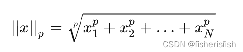，，其实是归一化操作，表示和这个向量方向相同的单位向量，这样的运算也叫向量的单位化。reshape作用不大，因为vierdirs本身是[1024,3]的矩阵

(64条消息) 机器学习中的范数规则化之（一）L0、L1与L2范数_l范数_zouxy09的博客-CSDN博客

    if use_viewdirs:# provide ray directions as inputviewdirs = rays_dif c2w_staticcam is not None:# special case to visualize effect of viewdirsrays_o, rays_d = get_rays(H, W, K, c2w_staticcam)viewdirs = viewdirs / torch.norm(viewdirs, dim=-1, keepdim=True)viewdirs = torch.reshape(viewdirs, [-1,3]).float()

 sh复制了rays_d的shape，值为torch.size([1024,3]),NDC坐标系可以参考大佬的文章

(64条消息) NeRF神经辐射场中关于光线从世界坐标系转换为NDC坐标系 Representing Scenes as Neural Radiance Fields for View Synthesis_出门吃三碗饭的博客-CSDN博客

    sh = rays_d.shape # [..., 3]if ndc:# for forward facing scenesrays_o, rays_d = ndc_rays(H, W, K[0][0], 1., rays_o, rays_d)

 这两个reshape作用同样不大，保持了矩阵大小一致

    # Create ray batchrays_o = torch.reshape(rays_o, [-1,3]).float()rays_d = torch.reshape(rays_d, [-1,3]).float()

 torch.ones_like函数和torch.zeros_like函数的基本功能是根据给定张量，生成与其形状相同的全1张量或全0张量，生成[1024,1]大小的near和far矩阵。torch.cat从列的维度拼接四个向量，最后形成[1024,8]的rays向量

    near, far = near * torch.ones_like(rays_d[...,:1]), far * torch.ones_like(rays_d[...,:1])rays = torch.cat([rays_o, rays_d, near, far], -1)

 再拼接上viewdirs，viewdirs 用于光线方向的单位化和位置编码,rays变成[1024,11]

    if use_viewdirs:rays = torch.cat([rays, viewdirs], -1)

 然后调用batchify_rays函数，核心目的是为了实现批量渲染，batchify_rays比较简单，rays_flat.shape[0]是1024，这里实际上只会进行一次循环，因为chunk是步长，一次就大于shape了，实际上chunk就是一次能进行渲染的光线最大值，这里设置成1024*32，所以rays_flat[i:i+chunk]其实就是输入的rays本身，只有rays更大的时候，chunk才会发挥作用，我们再来看这里引用的render_rays函数，

    # Render and reshapeall_ret = batchify_rays(rays, chunk, **kwargs)def batchify_rays(rays_flat, chunk=1024*32, **kwargs):"""Render rays in smaller minibatches to avoid OOM."""all_ret = {}for i in range(0, rays_flat.shape[0], chunk):ret = render_rays(rays_flat[i:i+chunk], **kwargs)for k in ret:if k not in all_ret:all_ret[k] = []all_ret[k].append(ret[k])all_ret = {k : torch.cat(all_ret[k], 0) for k in all_ret}return all_ret

 render_rays的输入输出，作者都解释的比较详细了，我们来一步步看看这些值是如何得到的

def render_rays(ray_batch,network_fn,network_query_fn,N_samples,retraw=False,lindisp=False,perturb=0.,N_importance=0,network_fine=None,white_bkgd=False,raw_noise_std=0.,verbose=False,pytest=False):"""Volumetric rendering.Args:ray_batch: array of shape [batch_size, ...]. All information necessaryfor sampling along a ray, including: ray origin, ray direction, mindist, max dist, and unit-magnitude viewing direction.network_fn: function. Model for predicting RGB and density at each pointin space.network_query_fn: function used for passing queries to network_fn.N_samples: int. Number of different times to sample along each ray.retraw: bool. If True, include model's raw, unprocessed predictions.lindisp: bool. If True, sample linearly in inverse depth rather than in depth.perturb: float, 0 or 1. If non-zero, each ray is sampled at stratifiedrandom points in time.N_importance: int. Number of additional times to sample along each ray.These samples are only passed to network_fine.network_fine: "fine" network with same spec as network_fn.white_bkgd: bool. If True, assume a white background.raw_noise_std: ...verbose: bool. If True, print more debugging info.Returns:rgb_map: [num_rays, 3]. Estimated RGB color of a ray. Comes from fine model.disp_map: [num_rays]. Disparity map. 1 / depth.acc_map: [num_rays]. Accumulated opacity along each ray. Comes from fine model.raw: [num_rays, num_samples, 4]. Raw predictions from model.rgb0: See rgb_map. Output for coarse model.disp0: See disp_map. Output for coarse model.acc0: See acc_map. Output for coarse model.z_std: [num_rays]. Standard deviation of distances along ray for eachsample.

首先就是将ray_batch 的输入分开拆出rays_o，rays_d，near，far 和 viewdirs，形状分别是[chunk, 3]，[chunk, 3]，[chunk, 1]，[chunk, 1] 和 [chunk, 3]。torch.reshape(ray_batch[...,6:8], [-1,1,2])其实就是将（1024，2），变成了（1024，1，2）

    N_rays = ray_batch.shape[0]rays_o, rays_d = ray_batch[:,0:3], ray_batch[:,3:6] # [N_rays, 3] eachviewdirs = ray_batch[:,-3:] if ray_batch.shape[-1] > 8 else Nonebounds = torch.reshape(ray_batch[...,6:8], [-1,1,2])near, far = bounds[...,0], bounds[...,1] # [-1,1]

 接下来的代码就要结合体渲染公式来看了，体渲染公式的讲解强烈推荐这篇大佬文章

“图形学小白”友好的NeRF原理透彻讲解 - 知乎 (zhihu.com)

若通过给定pose，从NeRF的模型中获得一张输出图片，关键就是获得每一个图片每一个像素坐标的像素值。在NeRF的paper中，给定一个camera pose，要计算某个像素坐标 (x,y) 的像素。通俗来说，该点的像素计算方法为：从相机光心发出一条射线（camera ray）经过该像素坐标，途径三维场景很多点，这些“途径点”或称作“采样点”的某种累加决定了该像素的最终颜色。

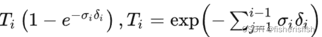
数学上，它的颜色由下面的“体渲染公式”计算而出，其中C表示渲染出的像素点颜色，σ表示体素密度， r 和 d 分别表示camera ray上的距离和ray上的方向，r=o+dt， t表示在camera ray上采样点离相机光心的距离，T表示透射比，也叫光学厚度、介质透明度，c表示当前区域的粒子发光和内散射辐射强度，也就是表面的实际颜色。

我们这里不再详提体渲染公式的推导过程，只看公式的代码实现。

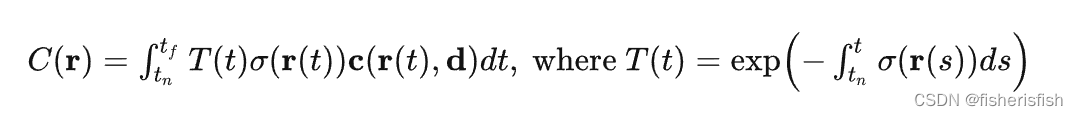
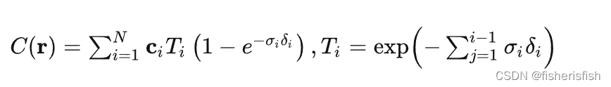
将 [tn, tf]均匀划分为 N个区间，并在这 N个区域内随机采样得到 N个采样点，即 ti(i=1,…,N)，进行求和得到颜色的估计值， σi和 δi分别表示当前区域粒子密度和区间步长 ，ci表示当前区域的粒子发光和内散射辐射强度， Ti表示透射比，括号中的公式表示透明度，公式没有考虑从相机发出的射线本身的强度。

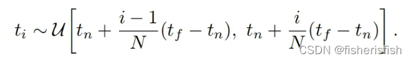
所以，  t_vals = torch.linspace(0., 1., steps=N_samples)相当于在（0，1）之间先均匀采样N个点，这里N_samples=64，lindisp是false，就是从深度采样，和公式是一样的。z_vals此时就是[1024,64]，expand之后没变化，此时的z_vals就是公式中的ti

    t_vals = torch.linspace(0., 1., steps=N_samples)if not lindisp:z_vals = near * (1.-t_vals) + far * (t_vals)else:z_vals = 1./(1./near * (1.-t_vals) + 1./far * (t_vals))z_vals = z_vals.expand([N_rays, N_samples])

接下来是均匀区间内随机产生采样点的过程，这里 perturb 默认值为1.0，并设 pytest 为 false，mids的形状为[chunk, N_samples-1]，即取N_samples的区间端点的中点，随后分别补充整个区间的上下界 tft_f 和 tnt_n ，得到 upper 和 lower 形状均为 [B, N_Sample] 。而随机数组 t_rand 的形状为 [chunk, N_samples] ，元素大小在[0, 1]。z_vals = lower + (upper - lower) * t_rand 计算出采样位置z_vals，形状为 [chunk, N_samples]。

但是，感觉这里存在一个小问题，z_vals 中的一个区间的 z_val 似乎只能取到原先区间的 [low, mid] 而不是 [low, up] ，假设每个区间的上下界和均值分别是up，low 和 mid 。

这里进行数据拼接 pts = rays_o[...,None,:] + rays_d[...,None,:] * z_vals[...,:,None]，pts 形状为 [chunk, N_samples, 3]。

(15 封私信 / 81 条消息) 为什么NeRF里可以仅凭位置和角度信息经过MLP预测出某点的rgb颜色？ - 知乎 (zhihu.com)

    if perturb > 0.:# get intervals between samplesmids = .5 * (z_vals[...,1:] + z_vals[...,:-1])upper = torch.cat([mids, z_vals[...,-1:]], -1)lower = torch.cat([z_vals[...,:1], mids], -1)# stratified samples in those intervalst_rand = torch.rand(z_vals.shape)# Pytest, overwrite u with numpy's fixed random numbersif pytest:np.random.seed(0)t_rand = np.random.rand(*list(z_vals.shape))t_rand = torch.Tensor(t_rand)z_vals = lower + (upper - lower) * t_randpts = rays_o[...,None,:] + rays_d[...,None,:] * z_vals[...,:,None] # [N_rays, N_samples, 3]

 搞到这里，迷惑的是这个pts是模型网络的输入，我们再来看一开始的模型，那么此时的pts是否是xyz，θ，φ呢？这里的输入其实是光线o+td，它的信息和xyz是一致的，代码里的None就是增加了一个为1的维度[1024,1,3]+[1024,1,3]*[1024,64,1]=[1024,64,3]？这一步矩阵乘法是怎么运算的？三维矩阵相乘时，前面的1024相同，不变，后面的[1,3]*[64,1]，这里发生的是广播逐元素相乘，如果是矩阵点乘numpy模块中矩阵乘法使用符号@，所以广播机制扩展成[64,3]*[64,3]，然后相加也是一样，广播成[1024,64,3]，广播的前提是有一个维度是1，这样子计算的物理含义是什么？1024代表了有N个射线，64代表了射线上的采样点的数量，3则是这些采样点的x,y,z坐标

  pts = rays_o[...,None,:] + rays_d[...,None,:] * z_vals[...,:,None] # [N_rays, N_samples, 3]

输入进入网络后，首先会被展开，变成了所有点的坐标[N_rands*N_samples,3]，然后所有点被送进了位置编码器embed_fn，之前提到过对位置编码的系数是10，输出维度是63，但是xyz的sin和cos只有60个输出，剩下3是什么？我们来看编码器创建的具体函数，这3其实就是输入的复制

    def create_embedding_fn(self):embed_fns = []d = self.kwargs['input_dims']out_dim = 0if self.kwargs['include_input']:embed_fns.append(lambda x : x)out_dim += d

def run_network(inputs, viewdirs, fn, embed_fn, embeddirs_fn, netchunk=1024*64):"""Prepares inputs and applies network 'fn'."""inputs_flat = torch.reshape(inputs, [-1, inputs.shape[-1]])embedded = embed_fn(inputs_flat)

然后是结合这个方向单位向量的代码，我其实很好奇这个的作用是什么，之前提到viewdirs 用于光线方向的单位化和位置编码，这里可以看出是给点的坐标加入了这个方向信息。那首先就是将输入的[1024,3]dirs扩展成[1024,64,3]，再同样展开成[1024*64,3]，然后我恍然大悟，原来viewdirs就是θ，φ信息， embeddirs_fn就是3+4*2*3，输出为[1024*64,27]，最后再和位置信息cat成[1024*64,90]

    if viewdirs is not None:input_dirs = viewdirs[:,None].expand(inputs.shape)input_dirs_flat = torch.reshape(input_dirs, [-1, input_dirs.shape[-1]])embedded_dirs = embeddirs_fn(input_dirs_flat)embedded = torch.cat([embedded, embedded_dirs], -1)

 输入终于理清之后，就到了网络前向推理的部分，fn即为NeRF的主体部分，chunk则是每次输入的大小设定，这里都是一次循环就结束了

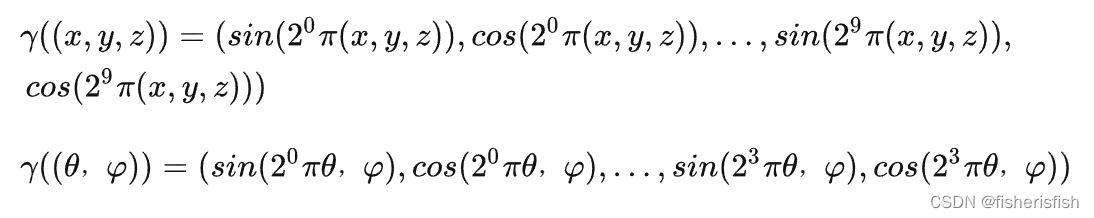
    outputs_flat = batchify(fn, netchunk)(embedded)def batchify(fn, chunk):"""Constructs a version of 'fn' that applies to smaller batches."""if chunk is None:return fndef ret(inputs):return torch.cat([fn(inputs[i:i+chunk]) for i in range(0, inputs.shape[0], chunk)], 0)return ret

 前向推理首先就是将位置和方向信息分开，这里input_ch和input_ch_views根据之前的定义分别是63和27，input_pts就是位置信息，这里直接进行了8层MLP计算，在第5层的时候（skips=4），又引入了一次input_pts，最终输出是[1024*64,256]，然后是对方向信息的特征提取，体素密度volume density（σ）层就直接输出，关键是rgb信息，首先h又经过了一层MLP，然后再引入input_views直接cat，再经过一层MLP将特征层缩小到128，最后再缩小到RGB3通道信息，最终RGB+σ作为输出返回，所以返回结果应该是[1024*64,4]

知乎大佬人累爱好者的模型图非常准确的反应了NeRF模型输入输出的关系，但是输入应该是63和27，而不是图中的60，24

    def forward(self, x):input_pts, input_views = torch.split(x, [self.input_ch, self.input_ch_views], dim=-1)h = input_ptsfor i, l in enumerate(self.pts_linears):h = self.pts_linears[i](h)h = F.relu(h)if i in self.skips:h = torch.cat([input_pts, h], -1)(pts_linears): ModuleList((0): Linear(in_features=63, out_features=256, bias=True)(1): Linear(in_features=256, out_features=256, bias=True)(2): Linear(in_features=256, out_features=256, bias=True)(3): Linear(in_features=256, out_features=256, bias=True)(4): Linear(in_features=256, out_features=256, bias=True)(5): Linear(in_features=319, out_features=256, bias=True)(6): Linear(in_features=256, out_features=256, bias=True)(7): Linear(in_features=256, out_features=256, bias=True))if self.use_viewdirs:alpha = self.alpha_linear(h)feature = self.feature_linear(h)h = torch.cat([feature, input_views], -1)for i, l in enumerate(self.views_linears):h = self.views_linears[i](h)h = F.relu(h)rgb = self.rgb_linear(h)(views_linears): ModuleList((0): Linear(in_features=283, out_features=128, bias=True))(feature_linear): Linear(in_features=256, out_features=256, bias=True)(alpha_linear): Linear(in_features=256, out_features=1, bias=True)(rgb_linear): Linear(in_features=128, out_features=3, bias=True)outputs = torch.cat([rgb, alpha], -1)else:outputs = self.output_linear(h)return outputs    

 在run_network函数里，还有最后一步就是将输出reshape成[1024,64,4]

    outputs = torch.reshape(outputs_flat, list(inputs.shape[:-1]) + [outputs_flat.shape[-1]])

推理完以后让我们再回到render_rays函数，在得到模型输出的raw之后，raw2outputs函数再得到各种结果图，raw2outputs的输入有raw，z_vals也就是64个采样点的间距信息，rays_d光线方向，raw_noise_std=0, white_bkgd=true, pytest=pytest

    raw = network_query_fn(pts, viewdirs, network_fn)rgb_map, disp_map, acc_map, weights, depth_map = raw2outputs(raw, z_vals, rays_d, raw_noise_std, white_bkgd, pytest=pytest)

raw2outputs函数首先就定义了raw2alpha函数，这个函数的作用就是求解之前的透明度， 定义了输入是raw，dists，act_fn，计算公式是同括号里的一致，但是加了一个激活函数F.relu，也就是保证raw是正值，然后此时的ci其实就是各点的RGB值，σi是网络输出的密度值， δi是计算得到的各点之间的步长dists，所以计算就豁然开朗了

def raw2outputs(raw, z_vals, rays_d, raw_noise_std=0, white_bkgd=False, pytest=False):"""Transforms model's predictions to semantically meaningful values.Args:raw: [num_rays, num_samples along ray, 4]. Prediction from model.z_vals: [num_rays, num_samples along ray]. Integration time.rays_d: [num_rays, 3]. Direction of each ray.Returns:rgb_map: [num_rays, 3]. Estimated RGB color of a ray.disp_map: [num_rays]. Disparity map. Inverse of depth map.acc_map: [num_rays]. Sum of weights along each ray.weights: [num_rays, num_samples]. Weights assigned to each sampled color.depth_map: [num_rays]. Estimated distance to object."""raw2alpha = lambda raw, dists, act_fn=F.relu: 1.-torch.exp(-act_fn(raw)*dists)

 dists变量其实是每两个点之间的距离，也就是[1024,63]，然后再加上一个最远的距离1e10，变成[1024,64]，然后再乘上方向向量rays_d的归一化向量，最后就变成在这个方向上的距离了。

    dists = z_vals[...,1:] - z_vals[...,:-1]dists = torch.cat([dists, torch.Tensor([1e10]).expand(dists[...,:1].shape)], -1)  # [N_rays, N_samples]dists = dists * torch.norm(rays_d[...,None,:], dim=-1)

 读取rgb信息，还用上了sigmoid，重新映射到[0,1]之间，这里如果要添加噪音的话会对alpha乘以噪音。

    rgb = torch.sigmoid(raw[...,:3])  # [N_rays, N_samples, 3]noise = 0.if raw_noise_std > 0.:noise = torch.randn(raw[...,3].shape) * raw_noise_std# Overwrite randomly sampled data if pytestif pytest:np.random.seed(0)noise = np.random.rand(*list(raw[...,3].shape)) * raw_noise_stdnoise = torch.Tensor(noise)

 根据之前的公式计算alpha

alpha = raw2alpha(raw[...,3] + noise, dists)

 weights值其实就是

• X = torch.ones((alpha.shape[0], 1))：X 是形状为 [1024, 1] 的全 1 矩阵
• Y = torch.cat([X, 1.-alpha + 1e-10], -1)：Y 是形状为 [1024, 64+1]，每行的第一个元素为全 1，后i个元素为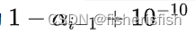
• cumprod为cumulative product的意思，即累积乘法。
• Z = torch.cumprod(Y, -1)：Z 是形状为 [1024, 64+1] 的连乘矩阵，除每行最后一个元素外，第 i个元素依次对应每条光线的 Ti 。

最终再和alpha相乘得到[1024,64]的weights，

weights = alpha * torch.cumprod(torch.cat([torch.ones((alpha.shape[0], 1)), 1.-alpha + 1e-10], -1), -1)[:, :-1]

 有了weights之后计算各种输出图，rgb_map就是weights乘以rgb后，再对64个点的rgb相加，得到最后的输出[1024,3]，depth_map就是这1024个点的深度值。

    rgb_map = torch.sum(weights[...,None] * rgb, -2)  # [N_rays, 3]depth_map = torch.sum(weights * z_vals, -1)disp_map = 1./torch.max(1e-10 * torch.ones_like(depth_map), depth_map / torch.sum(weights, -1))acc_map = torch.sum(weights, -1)rgb_map: [num_rays, 3]. Estimated RGB color of a ray.disp_map: [num_rays]. Disparity map. Inverse of depth map.acc_map: [num_rays]. Sum of weights along each ray.weights: [num_rays, num_samples]. Weights assigned to each sampled color.depth_map: [num_rays]. Estimated distance to object.if white_bkgd:rgb_map = rgb_map + (1.-acc_map[...,None])return rgb_map, disp_map, acc_map, weights, depth_map

再回到render_rays函数，N_importance=128，这里涉及到NeRF的Hierarchical volume sampling设计，首先使用分层抽样对第一组Nc位置进行采样，并在这些位置评估“粗糙”网络。给出这个“粗糙”网络的输出，然后我们对每条射线上的点进行更明智的采样，即利用反变换采样从这个分布中采样第二组Nf位置，然后将Nc+Nf采样得到的数据输入“精细”网络，并计算最终渲染的光线颜色C(r)。z_samples就是Nf的计算过程，sample_pdf函数就是反变换采样过程篇幅有限，后续再展开讲吧，detach 意为分离，对某个张量调用函数detach()，detach() 的作用是返回一个Tensor，它和原张量的数据相同，但requires_grad=False，也就意味着detach() 得到的张量不会具有梯度。这一性质即使我们修改其requires_grad 属性也无法改变。

    if N_importance > 0:rgb_map_0, disp_map_0, acc_map_0 = rgb_map, disp_map, acc_mapz_vals_mid = .5 * (z_vals[...,1:] + z_vals[...,:-1])z_samples = sample_pdf(z_vals_mid, weights[...,1:-1], N_importance, det=(perturb==0.), pytest=pytest)z_samples = z_samples.detach()z_vals, _ = torch.sort(torch.cat([z_vals, z_samples], -1), -1)pts = rays_o[...,None,:] + rays_d[...,None,:] * z_vals[...,:,None] # [N_rays, N_samples + N_importance, 3]run_fn = network_fn if network_fine is None else network_fine
#         raw = run_network(pts, fn=run_fn)raw = network_query_fn(pts, viewdirs, run_fn)rgb_map, disp_map, acc_map, weights, depth_map = raw2outputs(raw, z_vals, rays_d, raw_noise_std, white_bkgd, pytest=pytest)

 最终的结果采用粗精输出结合，返回这个ret，render_rays函数结束

    ret = {'rgb_map' : rgb_map, 'disp_map' : disp_map, 'acc_map' : acc_map}if retraw:ret['raw'] = rawif N_importance > 0:ret['rgb0'] = rgb_map_0ret['disp0'] = disp_map_0ret['acc0'] = acc_map_0ret['z_std'] = torch.std(z_samples, dim=-1, unbiased=False)  # [N_rays]

 再回到batchify_rays函数，因为chunk的设置只进行一次循环，所以all_ret和ret一致，batchify_rays函数结束，返回render函数

        ret = render_rays(rays_flat[i:i+chunk], **kwargs)for k in ret:if k not in all_ret:all_ret[k] = []all_ret[k].append(ret[k])all_ret = {k : torch.cat(all_ret[k], 0) for k in all_ret}return all_ret

 基本上就是返回最后的ret，变换了形式，直接贴结果，render函数结束，返回train函数

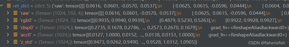
    # Render and reshapeall_ret = batchify_rays(rays, chunk, **kwargs)for k in all_ret:k_sh = list(sh[:-1]) + list(all_ret[k].shape[1:])all_ret[k] = torch.reshape(all_ret[k], k_sh)k_extract = ['rgb_map', 'disp_map', 'acc_map']ret_list = [all_ret[k] for k in k_extract]ret_dict = {k : all_ret[k] for k in all_ret if k not in k_extract}return ret_list + [ret_dict]

 train函数后续，后续其实就是常规的更新梯度并返回循环训练了。

        optimizer.zero_grad()#梯度归零img_loss = img2mse(rgb, target_s)#计算损失函数trans = extras['raw'][...,-1]loss = img_losspsnr = mse2psnr(img_loss)if 'rgb0' in extras:img_loss0 = img2mse(extras['rgb0'], target_s)loss = loss + img_loss0psnr0 = mse2psnr(img_loss0)loss.backward()optimizer.step()# NOTE: IMPORTANT!###   update learning rate   ###decay_rate = 0.1decay_steps = args.lrate_decay * 1000new_lrate = args.lrate * (decay_rate ** (global_step / decay_steps))for param_group in optimizer.param_groups:param_group['lr'] = new_lrate################################dt = time.time()-time0

本文来自互联网用户投稿，文章观点仅代表作者本人，不代表本站立场，不承担相关法律责任。如若转载，请注明出处。 如若内容造成侵权/违法违规/事实不符，请点击【内容举报】进行投诉反馈！