python 排序统计滤波器_马尔可夫链+贝叶斯滤波器的Python展示

知乎上已经有很多的学习笔记，但读完后总有一种这东西不是我的我理解不了的感觉，所以想试着写一篇文章来加深一下自己的理解，也记录下学习中的盲点。

非常推荐大家去Github看一个项目：

#下面的代码也是完全基于上述作者的库函数完成的，所以需要先去Github下载库函数安装,或者直接使用
pip install filterpy
#但是作者忘记把离散的白噪声函数放进库里，那段函数可以在书里找到，或者改天我可以放在网盘里分享出来
#不影响下面代码展示

这里除了有卡尔曼滤波外还有各种贝叶斯滤波的python实现，作者也写了一本书开源在Github详细介绍了卡尔曼，本文就算是读书笔记吧。下面是作者发布的教材：

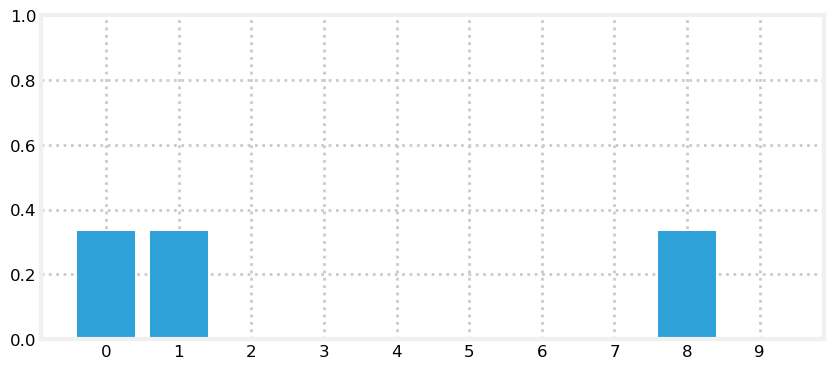
太高估自己的效率，听了128次大田后生仔+n首其他终于赶在没有眼瞎前停工了。

下面代码基本是从原作者书里粘来的，我只改了某些错误和可视化以及一些小的细节（动图做的还不够好）作者在书中试图用追踪狗在走廊中移动的模型来解释离散贝叶斯滤波，由先验概率到后验概率再到引入反馈器这一思路详细的介绍了贝叶斯滤波器并且实现了python的编程。同时作者一直在向我们强调学会数学编程的重要性，本人理解的不够深刻，大家可以去翻阅原作者的书去看。

为什么我一直想实现贝叶斯滤波或者卡尔曼滤波，因为它是一种动态滤波器，它可以用来建立动态的反演模型，这和我以前接触的反演很不一样，我曾经做过利用光学遥感建立泥沙反演模型和利用两层BP神经网络对地震波建立反演模型找地下矿层的两个小东西，以上两个反演模型都是静态的过程，而卡尔曼滤波最反智的则是在滤波中不断更新模型参数（加入了后馈过程也就是K卡尔曼增益矩阵），这让我困惑了特别久。

如果大家也对这种滤波器感兴趣建议先学些统计知识和最小二乘法，卡尔曼滤波和最小二乘法之间有着很紧密地联系，并且最小二乘法方程可以很好的帮助你理解最小均方误差，这是实现卡尔曼滤波的重要假设。

下面也会放一段简单马尔可夫链的python小程序，如果你和我一样用Sublime ，多试几次Ctrl + B，这是基于随机数做的，但是你会发现在多次迭代后概率会收敛到一个定值，还记得统计课上讲的大数定律嘛，在样本空间足够大时，依概率收敛到某个数，大约就是这个意思。所以在随机天气生成器中需要用蒙托卡罗思想来添加扰动来破坏这种收敛性？，我上一篇文章中也写道过，但是我想错了，并不是对转移概率矩阵添加扰动，而是对初始状态添加扰动（最近听了几个MCMC方法的读书汇报，发现了这个秘密）

有关于今天统计课上讲到的气候序列均一化我也想说点儿给某位不来上课的同学，我认为卡尔曼滤波器可以很好的应用到均一化过程中，具体方法我不说，啦啦啦。

#离散贝叶斯滤波器的实现展示
#The Kalman filter belongs to a family of filters called Bayesian filters.
#NMEFC YuHao
import numpy as np
import matplotlib.pyplot as plt
from filterpy.discrete_bayes import normalize
from filterpy.discrete_bayes import predict
from filterpy.discrete_bayes import updatex = range(10)
hallway = np.array([1,1,0,0,0,0,0,0,1,0])
#Tracking a Dogdef update_belief(hall,belief,z,correct_scale):for i ,val in enumerate(hall):if val == z:belief[i] *= correct_scale
belief = np.array([0.1]*10)
reading = 1
update_belief(hallway,belief,z = reading,correct_scale = 3.)
print("belief:",belief)
print("sum = ",sum(belief))
plt.figure()
plt.bar(x,belief)
plt.title("belief")
plt.show()#归一化
homogeneity_array = belief/sum(belief)
print(homogeneity_array)
print(hallway == 1 )
#计算后验概率
def scale_update(hall ,belief, z, z_prob):scale = z_prob / (1. - z_prob)belief[hall == z] *= scalenormalize(belief)
belief = np.array([0.1]*10)
scale_update(hallway ,belief ,z=1,z_prob = .75)
print('sum =',sum(belief))
print("probability of door =",belief[0])
print("probability of wall =", belief[2])
plt.figure()
plt.bar(x,belief)
plt.title("belief")
plt.show()def scale_update(hall,belief,z,z_prob):scale = z_prob / (1. - z_prob)likelihood = np.ones(len(hall))likelihood[hall == z] *= scalereturn normalize(likelihood * belief)
def lh_hallway(hall, z, z_prob):#compute likelihood that a measurement matches#positions in the hallway.try:scale = z_prob / (1. - z_prob)except ZeroDivisionError:scale = 1e8likelihood = np.ones(len(hall))likelihood[hall==z] *= scalereturn likelihoodbelief = np.array([0.1] * 10)
likelihood = lh_hallway(hallway, z=1, z_prob=.75)
print(normalize(likelihood * belief))  
def perfect_predict(belief,move):n = len(belief)result = np.zeros(n)for i in range(n):result[i] = belief[(i-move) % n]return result
belief = np.array([.35,.1,.2,.3,0,0,0,0,0,.05])belief = perfect_predict(belief,1)
plt.bar(x,belief)
plt.title("belief")
plt.show()
#添加噪声def predict_move(belief, move, p_under, p_correct, p_over):n = len(belief)prior = np.zeros(n)for i in range(n):prior[i] = (belief[(i-move) % n]   * p_correct +belief[(i-move-1) % n] * p_over +belief[(i-move+1) % n] * p_under)      return priorbelief = [0., 0., 0., 1., 0., 0., 0., 0., 0., 0.]
prior = predict_move(belief, 2, .1, .8, .1)
print(prior)
fig = plt.figure()
ax1 = fig.add_subplot(1,2,1)
ax2 = fig.add_subplot(1,2,2)
ax1.bar(x,belief)
ax2.bar(x,prior)
ax1.set_title("belief")
ax2.set_title("prior")
ax1.set_xticks(x)
ax2.set_xticks(x)
plt.show()
belief = [0, 0, .4, .6, 0, 0, 0, 0, 0, 0]
prior = predict_move(belief, 2, .1, .8, .1)
fig = plt.figure()
ax1 = fig.add_subplot(1,2,1)
ax2 = fig.add_subplot(1,2,2)
ax1.bar(x,belief)
ax2.bar(x,prior)
ax1.set_title("belief")
ax2.set_title("prior")
ax1.set_xticks(x)
ax2.set_xticks(x)
plt.show()belief = np.array([1.0,0,0,0,0,0,0,0,0,0])
beliefs = []
for i in range(100):belief = predict_move(belief,1,.1,.8,.1)beliefs.append(belief)
print("Final Belief:",belief)
print(len(beliefs))
print(beliefs[1])
for i in range(len(beliefs)):plt.cla()plt.bar(x,beliefs[i])plt.xticks(x)plt.pause(0.05)plt.show()
"""
#卷积泛化
#卷积算法的python描述，但是时间复杂度太高，pass
def predict_move_convolution(pdf ,offset,kernel):N = len(pdf)kN = len(kernel)width = int((kN - 1)/2)prior = np.zeros(N)for i in range(N):for k in range(kN):index = (i + (width - k)-offset)%Nprior[i] += pdf[index] * kernel[k]return prior
"""belief = [.05, .05, .05, .05, .55, .05, .05, .05, .05, .05]
prior = predict(belief,offset = 1,kernel = [.1,.8,.1])
fig = plt.figure()
ax1 = fig.add_subplot(1,2,1)
ax2 = fig.add_subplot(1,2,2)
ax1.bar(x,belief)
ax2.bar(x,prior)
ax1.set_title("belief")
ax2.set_title("prior")
ax1.set_xticks(x)
ax2.set_xticks(x)
plt.show()
prior = predict(belief, offset=3, kernel=[.05, .05, .6, .2, .1])
#make sure that it shifts the positions correctly for movements greater than one and for asymmetric kernels
#making a prediction of where the dog is moving, and convolving the probabilities to get the priorfig = plt.figure()
ax1 = fig.add_subplot(1,2,1)
ax2 = fig.add_subplot(1,2,2)
ax1.bar(x,belief)
ax2.bar(x,prior)
ax1.set_title("belief")
ax2.set_title("prior")
ax1.set_xticks(x)
ax2.set_xticks(x)
plt.show()
"""
#Integrating Measurements and Movement Updates
"""
"""
请仔细阅读下一段话
Let's think about this intuitively.Consider a simple case - you are tracking a dog while he sits still.During each prediction you predict he doesn't move.Your filter quickly converges on an accurate estimate of his position.Then the microwave in the kitchen turns on, and he goes streaking off.You don't know this, so at the next prediction you predict he is in the same spot.But the measurements tell a different story.As you incorporate the measurements your belief will be smeared along the hallway, leading towards the kitchen.On every epoch (cycle) your belief that he is sitting still will get smaller,and your belief that he is inbound towards the kitchen at a startling rate of speed increases.
最精彩的部分来了：反馈器"""
tank1 = []
tank2 = []hallway = np.array([1, 1, 0, 0, 0, 0, 0, 0, 1, 0])
prior = np.array([.1] * 10)
likelihood = lh_hallway(hallway, z=1, z_prob=.75)
posterior = normalize(likelihood * prior)
tank2.append(posterior)
tank1.append(prior)
fig = plt.figure()
ax1 = fig.add_subplot(1,2,1)
ax2 = fig.add_subplot(1,2,2)
ax1.bar(x,prior)
ax2.bar(x,posterior)
ax1.set_title("prior")
ax2.set_title("posterior")
ax1.set_xticks(x)
ax1.set_ylim(0,0.5)
ax2.set_ylim(0,0.5)
ax2.set_xticks(x)
plt.show()#After the first update we have assigned a high probability to each door position, and a low probability to each wall position.
prior = np.array([.1] * 10)
kernel = (.1, .8, .1)
prior = predict(posterior, 1, kernel)
tank1.append(posterior)
tank2.append(prior)
fig = plt.figure()
ax1 = fig.add_subplot(1,2,1)
ax2 = fig.add_subplot(1,2,2)
ax1.bar(x,prior)
ax2.bar(x,posterior)
ax1.set_title("posterior")
ax2.set_title("prior")
ax1.set_xticks(x)
ax1.set_ylim(0,0.5)
ax2.set_ylim(0,0.5)
ax2.set_xticks(x)
plt.show()
#The predict step shifted these probabilities to the right, smearing them about a bit. Now let's look at what happens at the next sense.likelihood = lh_hallway(hallway, z=1, z_prob=.75)
posterior = update(likelihood, prior)
tank1.append(prior)
tank2.append(posterior)
fig = plt.figure()
ax1 = fig.add_subplot(1,2,1)
ax2 = fig.add_subplot(1,2,2)
ax1.bar(x,prior)
ax2.bar(x,posterior)
ax1.set_title("prior")
ax2.set_title("posterior")
ax1.set_xticks(x)
ax1.set_ylim(0,0.5)
ax2.set_ylim(0,0.5)
ax2.set_xticks(x)
plt.show()
#Notice the tall bar at position 1. This corresponds with the (correct) case of starting at position 0, sensing a door, shifting 1 to the right, and sensing another door. No other positions make this set of observations as likely. Now we will add an update and then sense the wall.
prior = predict(posterior, 1, kernel)
likelihood = lh_hallway(hallway, z=0, z_prob=.75)
posterior = update(likelihood, prior)
tank1.append(prior)
tank2.append(posterior)
fig = plt.figure()
ax1 = fig.add_subplot(1,2,1)
ax2 = fig.add_subplot(1,2,2)
ax1.bar(x,prior)
ax2.bar(x,posterior)
ax1.set_title("prior")
ax2.set_title("posterior")
ax1.set_xticks(x)
ax1.set_ylim(0,0.5)
ax2.set_ylim(0,0.5)
ax2.set_xticks(x)
plt.show()
#This is exciting! We have a very prominent bar at position 2 with a value of around 35%. It is over twice the value of any other bar in the plot, and is about 4% larger than our last plot, where the tallest bar was around 31%. Let's see one more cycle.
prior = predict(posterior, 1, kernel)
likelihood = lh_hallway(hallway, z=0, z_prob=.75)
posterior = update(likelihood, prior)
prior = predict(posterior, 1, kernel)
likelihood = lh_hallway(hallway, z=0, z_prob=.75)
posterior = update(likelihood, prior)
tank1.append(prior)
tank2.append(posterior)
fig = plt.figure()
ax1 = fig.add_subplot(1,2,1)
ax2 = fig.add_subplot(1,2,2)
ax1.bar(x,prior)
ax2.bar(x,posterior)
ax1.set_title("prior")
ax2.set_title("posterior")
ax1.set_xticks(x)
ax1.set_ylim(0,0.5)
ax2.set_ylim(0,0.5)
ax2.set_xticks(x)
plt.show()
print(tank1)
print(tank2)
for i in range(len(tank1)):plt.cla()plt.subplot(1,2,1)plt.bar(x,tank1[i])plt.xticks(x)plt.ylim(0,0.5)plt.subplot(1,2,2)plt.bar(x,tank2[i])plt.xticks(x)plt.ylim(0,0.5)plt.pause(0.5)plt.show()
#离散贝叶斯算法

备注添加的可能不是很准确，有问题大家可以留言。

import numpy as np
import random as rmstate = ["sleep","Icecream","Run"]
transitionName = [["SS","SR","SI"],["RS","RR","RI"],["IS","IR","II"]]
transitionMatrix = [[0.2,0.6,0.2],[0.1,0.6,0.3],[0.2,0.7,0.1]]
if sum(transitionMatrix[0]) + sum(transitionMatrix[1]) + sum(transitionMatrix[2]) !=3:print("Wrong")
else:print("All is gonna be okay,you should move on!!;)")def activity_forecast(days):activityToday = "Sleep"#print("Start_state:" + activityToday)activityList = [activityToday]i = 0prob = 1while i != days:if activityToday == "Sleep":change = np.random.choice(transitionName[0],replace = True,p =transitionMatrix[0])if change == "SS":prob = prob * 0.2activityList.append("Sleep")passelif change == "SR":prob = prob * 0.6activityToday = "Sleep"activityList.append("Sleep")else:prob = prob *0.2activityToday = "Icecream"activityList.append("Icecream")elif activityToday == "Run":change = np.random.choice(transitionName[1],replace = True ,p = transitionMatrix[1])if change == "RR":prob = prob * 0.5activityList.append("Run")passelif change == "RS":prob = prob *0.2activityToday = "Sleep"activityList.append("Sleep")else:prob = prob * 0.3activityToday = "Icecream"activityList.append("Icecream")elif activityToday == "Icecream":change = np.random.choice(transitionName[2],replace = True,p = transitionMatrix[2])if change == "II":prob = prob *0.1activityList.append("Icecream")passelif change == "IS":prob = prob * 0.2activityToday = "Sleep"activityList.append("Sleep")else:prob = prob * 0.7activityToday = "Run"activityList.append("Run")i += 1return activityList
list_activity = []
count = 0
for iterations in range(1,10000):list_activity.append(activity_forecast(2))
for smaller_list in list_activity:if(smaller_list[2] == "Sleep"):count += 1
percentage = (count/10000) * 100print("the probability of starting at state:'Sleep' and ending at state:'Sleep' = " + str(percentage) + "%")#马尔可夫链展示

能看到这儿说明你对我的文章很有兴趣，那么有任何问题可以通过任何方式问我。

日常吐槽：

最近效率真是低的可怕，可我睡不着啊。。。

休息不好吃又吃不下要掉体重了，为了回家不让老妈发现（不然要被疯狂投食）牛奶得换全脂来保证热量摄入了。

来吧，都看到这儿了陪我听首歌啊：

柯姓男孩永不认输

本文来自互联网用户投稿，文章观点仅代表作者本人，不代表本站立场，不承担相关法律责任。如若转载，请注明出处。 如若内容造成侵权/违法违规/事实不符，请点击【内容举报】进行投诉反馈！