提示：文章写完后，目录可以自动生成，如何生成可参考右边的帮助文档

CNN卷积神经网络

• 前言
• 一、CNN是什么？
• 二、为什么要使用CNN？
• 三、CNN的结构
• • 1.图片的结构
  • 2.卷积层
  • • 1.感受野（Receptive Field）
    • 2.卷积层的输出
    • 3.权值共享
  • 3.池化层(pooling)
  • 4.全连接层
• 四、ICS(Internal Covariate shift)
• • 1.ICS是什么？
  • 2.ICS导致的问题
  • 3.ICS的解决方法
  • • 1.白化(whiting)
    • 2.正则化(normalization)
    • 3.Batch Normalization
• 五、作业代码详解
• • 1.题目要求
  • 2.引入库
  • 3.构造数据集
  • 4.CNN模型构造
  • 5.参数准备
  • 6.训练模型
  • 7.测试数据
• 总结

前言

由这篇文章开始，我们正式进入算法方面的介绍，这一篇文章将会介绍CNN卷积神经网络

一、CNN是什么？

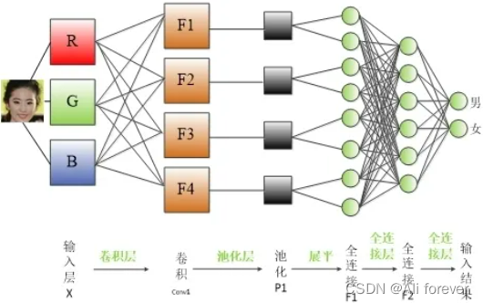
卷积神经网络是一类包含卷积计算且具有深度结构的前馈神经网络，其默认输入是图像(image),结构分为三层，分别是卷积层，池化层，全连接层，他们共同构成了CNN卷积神经网络。

二、为什么要使用CNN？

在之前的深度学习模型，我们介绍了全连接神经网络模型，全连接神经网络模型的特点就是下一层的每一个神经元都需要与上一层的所有神经元全部遍历连接，这样会产生非常多的权重$w$，过多的权重参数$w$会带来以下几个缺点:

1. 过多的参数会导致训练效率低下，时间很长
2. 过多的参数会导致过拟合的风险
3. 全连接神经网络将特征展平后占用过多的空间，有可能导致空间不够而丢失空间信息

而CNN则有以下优点:

1. 共享卷积核，处理高维数据无压力
2. 可以自动进行特征提取

所以可以看出CNN能解决掉全连接神经网络中参数过多的缺点，共享参数。
但事实上CNN也有以下几个缺点:

1. 采用梯度下降算法很容易使训练结果收敛于局部最小值而非全局最小值
2. 池化层会丢失大量有价值信息，忽略局部与整体之间关联性
3. 由于特征提取的封装，为网络性能的改进罩了一层黑盒
4. 当网络层次太深时，采用BP传播修改参数会使靠近输入层的参数改动较慢

三、CNN的结构

1.图片的结构

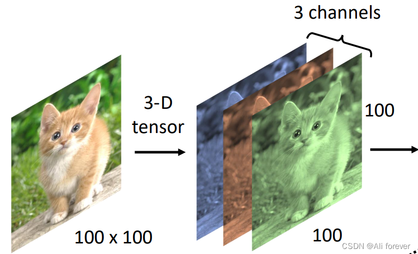
当图片进行输入时，我们可以把图片看成是一张长*宽的矩阵，但是事实上图片是一个三维的tensor，他还会有三个channel，分别是red，green，blue。

所以事实上，我们的神经元并不需要遍历整个图片，而是负责其中的一部分就可以辨认出图片的特征。

2.卷积层

所谓的卷积，就是两个函数进行叠加操作。而这里的卷积可以认同为，则可以理解对图像进行滤波操作，重点突出图像中的某些特征，删除某些无关紧要的特征，并且可以降低参数的数量

1.感受野（Receptive Field）

我们前面说过，我们只需要神经元与图片的一部分做连接，这个连接的区域我们就叫他感受野，他的尺寸形状不固定，大小也不固定，是一个超参数，需要我们手动调整。但是这个感受野的深度，一般与channel的长度相同

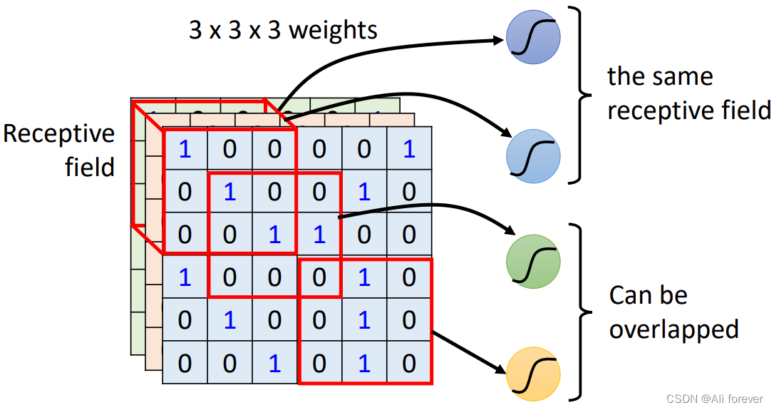
感受野的设置不能过大，否则训练的参数都是对应于整个对象的局部信息，是不够利于检测大小目标的。如果感受野的设置过小，训练参数只有少部分是对应于训练目标的，则在测试环节，也很难检测出类似的目标。

2.卷积层的输出

我们可以看到每个卷积核之间是有重叠的，这是因为如果卷积核之间没有重叠的话，相邻地输出将会没有意义，而我们需要通过多个卷积核的输出去判定图像的特征，所以这样是不行的。所以我们引入了步长(stride)，但是步长的设置不能随便确定，需要保证卷积核平滑地扫过整个感知域，他的取值还受限于padding跟卷积核的大小

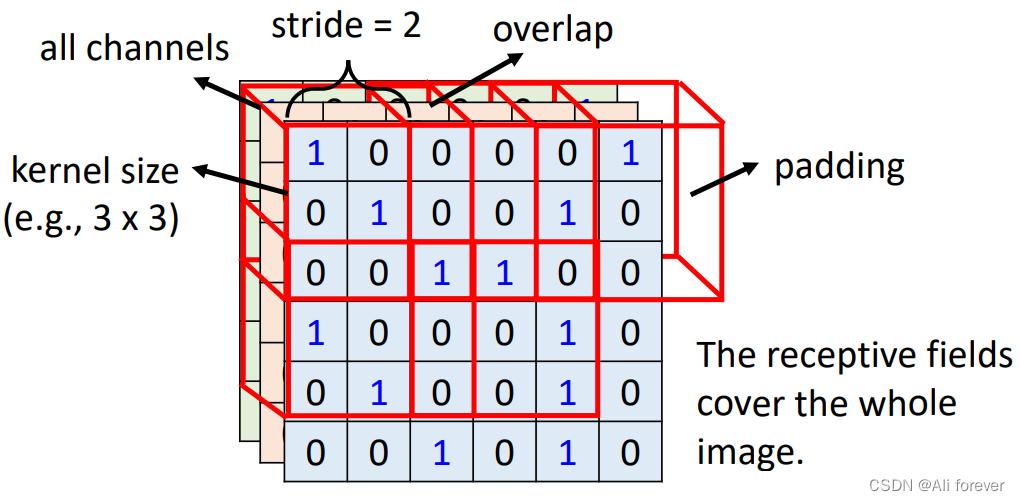
为了能让卷积核平滑地扫过，以致于在边缘不缺失取值，控制输出的尺寸，我们必须要引入填充(padding),一般我们是采取零填充，这样会比较常见，当然我们也可以引入平均值填充，这取决与我们的需要
下面还有计算输出层宽度大小的公式:
W n e x t = ( W n o w − F + 2 P ) S + 1 W_{next} =\frac{(W_{now}-F+2P)}{S}+1 Wnext​=S(Wnow​−F+2P)​+1
其中S是步长，F是卷积核的大小，P是填充大小

3.权值共享

由于同一个特征在不同的感知域中其实检测的效果都相同，如果不同的感受野中都要设置不同权值去进行卷积核的计算，那样参数就过于多，过于复杂了，所以我们会采用权值共享，则不同感受野中的卷积核都是一样的。

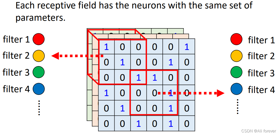
使用权值共享后，每一个卷积核只能提取出一个特征，所以我们在每个感受野中需要多个不同的卷积核，而不同深度的神经也会有不同的权重集

3.池化层(pooling)

相邻地两个卷积层中会周期地插入池化层，通过池化来进一步降低图片的尺寸。

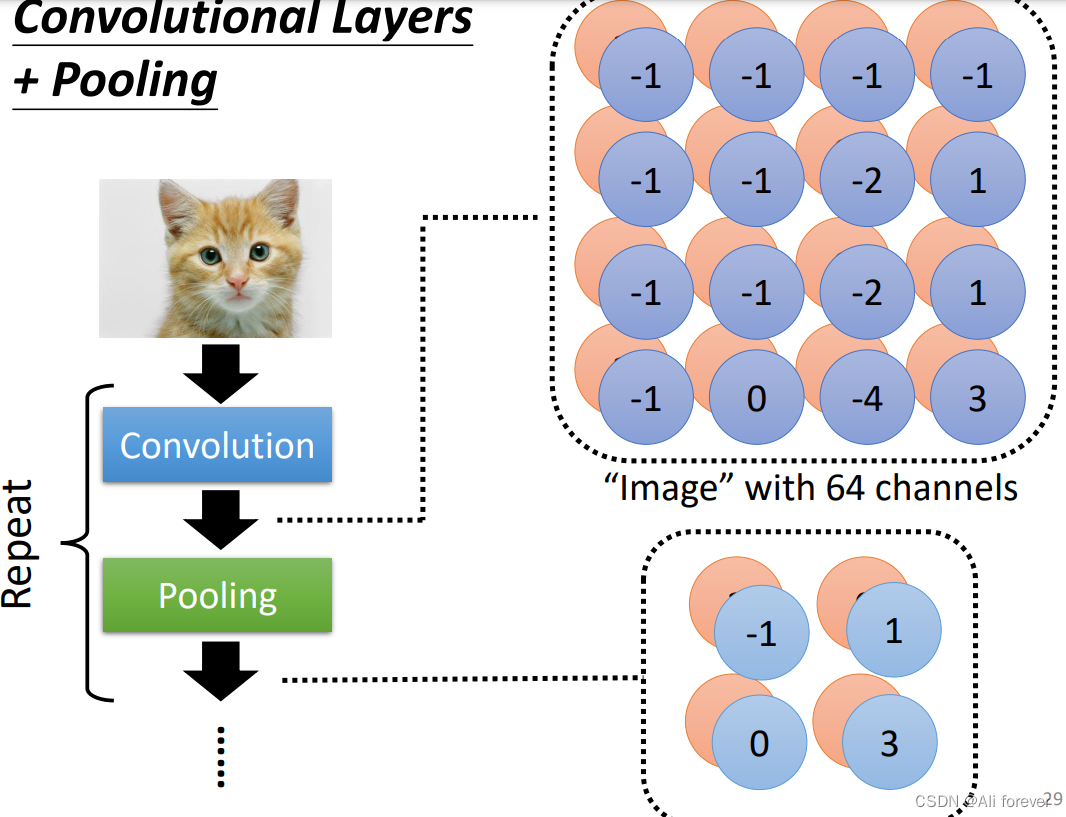
池化层一般采用的是对一张大的图片做subsampling(下采样)，先设定一个汇聚层，然后在汇聚的范围里面取值最大的一个代表这一个部分，但是channel不会改变。
但事实上，CNN并不能对图片进行放大缩小，旋转等操作，这些需要用到图像增强才可以。
下面还有池化层计算输出层宽度大小的公式:
W n e x t = ( W n o w − F ) S + 1 W_{next} =\frac{(W_{now}-F)}{S}+1 Wnext​=S(Wnow​−F)​+1
其中S是步长，F是池化层的大小

4.全连接层

在卷积层的最后，我们一般会设置一个全连接层，将卷积层转化为全连接层。全连接层的权重是一个巨大的矩阵，除了某些特定块（感受野），其余部分都是零；而在非 0 部分中，大部分元素都是相等的（权值共享）

四、ICS(Internal Covariate shift)

1.ICS是什么？

深度神经网络涉及到很多层的叠加，而每一层的参数更新会导致上层的输入数据分布发生变化，层层叠加后，高层的输入分布变化会很明显，使得高层需要重新适应底层的参数更新。这种问题我们就称为ICS问题。

2.ICS导致的问题

ICS会导致上层网络需要不断适应新的输入数据分布，降低学习速度。下层输入的变化可能趋向于变大或者变小，导致上层落入饱和区，使得学习过早停止。每层的更新都会影响到其它层，因此每层的参数更新策略需要尽可能的谨慎。

3.ICS的解决方法

解决ICS最直接的思想就是使每层的分布都是独立同分布

1.白化(whiting)

白化是对输入数据分布进行变换，进而达到以下两个目的：

1. 使得输入特征分布具有相同的均值与方差，其中PCA白化保证了所有特征分布均值为0，方差为1；而ZCA白化则保证了所有特征分布均值为0，方差相同；
2. 去除特征之间的相关性。

但是白化的计算成本太高，不适宜在大规模计算中使用

2.正则化(normalization)

Normalization则是把分布强行拉回到均值为0方差为1的标准正态分布，使得激活输入值落在非线性函数对输入比较敏感的区域，这样输入的小变化就会导致损失函数较大的变化，避免梯度消失问题产生，加速收敛.
但如果使用标准化，那就相当于把非线性激活函数替换成线性函数了，这样不利用复杂模型的建立，容易造成model bias。

3.Batch Normalization

标准化针对输入数据的单一维度进行，根据每一个batch计算均值与标准差，由于从形象上是纵向的计算，又称为纵向标准化

五、作业代码详解

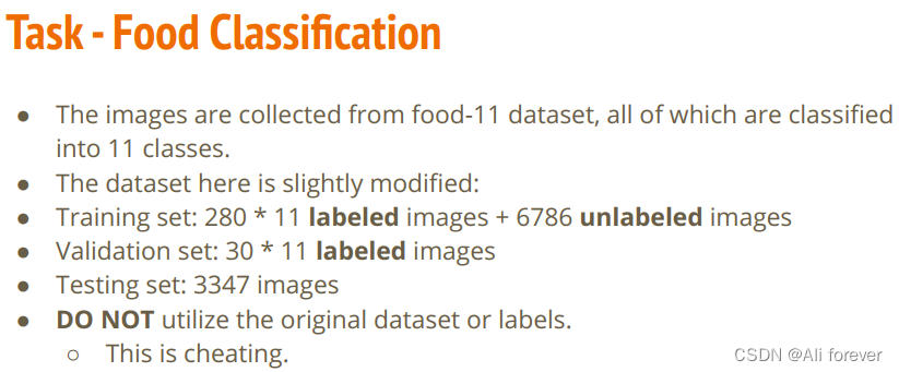
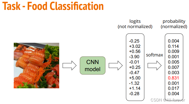
1.题目要求

2.引入库

# Import necessary packages.
import numpy as np
import torch
import torch.nn as nn
import torchvision.transforms as transforms
from PIL import Image
# "ConcatDataset" and "Subset" are possibly useful when doing semi-supervised learning.
from torch.utils.data import ConcatDataset, DataLoader, Subset
from torchvision.datasets import ImageFolder
# This is for the progress bar.
from tqdm.auto import tqdm

torchvision包: torchvision是pytorch的一个图形库，它服务于PyTorch深度学习框架的，主要用来构建计算机视觉模型。以下是torchvision的构成：
torchvision.transforms:常用的图片变换，例如裁剪、旋转等
torchvision.datasets:一些加载图片数据的函数及常用的数据集接口
torchvision.models: 包含常用的模型结构（含预训练模型），例如AlexNet、VGG、ResNet等

3.构造数据集

train_trm=transforms.Compose([transforms.Resize(128,128),transforms.ToTensor(),])
test_trm=transforms.Compose([transforms.Resize(128,128),transforms.ToTensor(),])batch_size=128
train_set=ImageFolder("food-11/training/labeled", transform=train_tfm)
valid_set=ImageFolder("food-11/validation", transform=test_tfm)
unlabeled_set = ImageFolder("food-11/training/unlabeled",  transform=train_tfm)
test_set = ImageFolder("food-11/testing", transform=test_tfm)train_loader=DataLoader(train_set,batch_size=batch_size,shuffle=True,num_work=0,pin_memory=True)
valid_loader=DataLoader(valid_set,batch_size=batch_size,shuffle=True,num_work=0,pin_memory=True)
test_loader=DataLoader(test_set,batch_size=batch_size,shuffle=False)

transforms.Compose:这个类的主要作用是串联多个图片变换的操作,可以看到这个类的内容是一个列表，将会遍历列表进行操作。
transforms.Resize(128,128),transforms.ToTensor():前面是将PIL图片的维度改变，然后最后将PIL图片改变为一张Tensor向量。
torchvision.datasets.ImageFolder(root, transform=None, target_transform=None, loader=, is_valid_file=None):是一个容器,
root:图片存储的根目录，即各类别文件夹所在目录的上一级目录。
transform:对图片进行预处理的操作函数,原始图片作为输入,返回一个转换后的图片,
target_transform：对图片类别进行预处理的操作，输入为 target，输出对其的转换。 如果不传该参数，即对 target 不做任何转换，返回的顺序索引 0,1, 2…

4.CNN模型构造

在处理好进来的数据集后，我们将会搭建我们的CNN模型，我们可以看到用到了nn.BatchNorm2d解决ICS问题

class Classifier(nn.Module):def __init__(self):super(Classifier, self).__init__()# The arguments for commonly used modules:# torch.nn.Conv2d(in_channels, out_channels, kernel_size, stride, padding)# torch.nn.MaxPool2d(kernel_size, stride, padding)# input image size: [3, 128, 128]self.cnn_layers = nn.Sequential(nn.Conv2d(3, 64, 3, 1, 1),nn.BatchNorm2d(64),nn.ReLU(),nn.MaxPool2d(2, 2, 0),nn.Conv2d(64, 128, 3, 1, 1),nn.BatchNorm2d(128),nn.ReLU(),nn.MaxPool2d(2, 2, 0),nn.Conv2d(128, 256, 3, 1, 1),nn.BatchNorm2d(256),nn.ReLU(),nn.MaxPool2d(4, 4, 0),)print()self.fc_layers = nn.Sequential(nn.Linear(256 * 8 * 8, 256),nn.ReLU(),nn.Linear(256, 256),nn.ReLU(),nn.Linear(256, 11))def forward(self, x):# input (x): [batch_size, 3, 128, 128]# output: [batch_size, 11]# Extract features by convolutional layers.x = self.cnn_layers(x)# The extracted feature map must be flatten before going to fully-connected layers.x = x.flatten(1)# The features are transformed by fully-connected layers to obtain the final logits.x = self.fc_layers(x)return x

5.参数准备

# "cuda" only when GPUs are available.
device = "cuda" if torch.cuda.is_available() else "cpu"# Initialize a model, and put it on the device specified.
model = Classifier().to(device)
model.device = device# For the classification task, we use cross-entropy as the measurement of performance.
criterion = nn.CrossEntropyLoss()# Initialize optimizer, you may fine-tune some hyperparameters such as learning rate on your own.
optimizer = torch.optim.Adam(model.parameters(), lr=0.0003, weight_decay=1e-5)# The number of training epochs.
n_epochs = 80

6.训练模型

for epoch in range(n_epochs):# ---------- Training ----------# Make sure the model is in train mode before training.model.train()# These are used to record information in training.train_loss = []train_accs = []# Iterate the training set by batches.for batch in tqdm(train_loader):# A batch consists of image data and corresponding labels.imgs, labels = batch# Forward the data. (Make sure data and model are on the same device.)logits = model(imgs.to(device))# Calculate the cross-entropy loss.# We don't need to apply softmax before computing cross-entropy as it is done automatically.loss = criterion(logits, labels.to(device))# Gradients stored in the parameters in the previous step should be cleared out first.optimizer.zero_grad()# Compute the gradients for parameters.loss.backward()# Clip the gradient norms for stable training.grad_norm = nn.utils.clip_grad_norm_(model.parameters(), max_norm=10)# Update the parameters with computed gradients.optimizer.step()# Compute the accuracy for current batch.acc = (logits.argmax(dim=-1) == labels.to(device)).float().mean()# Record the loss and accuracy.train_loss.append(loss.item())train_accs.append(acc)# The average loss and accuracy of the training set is the average of the recorded values.train_loss = sum(train_loss) / len(train_loss)train_acc = sum(train_accs) / len(train_accs)# Print the information.print(f"[ Train | {epoch + 1:03d}/{n_epochs:03d} ] loss = {train_loss:.5f}, acc = {train_acc:.5f}")# ---------- Validation ----------# Make sure the model is in eval mode so that some modules like dropout are disabled and work normally.model.eval()# These are used to record information in validation.valid_loss = []valid_accs = []# Iterate the validation set by batches.for batch in tqdm(valid_loader):# A batch consists of image data and corresponding labels.imgs, labels = batch# We don't need gradient in validation.# Using torch.no_grad() accelerates the forward process.with torch.no_grad():logits = model(imgs.to(device))# We can still compute the loss (but not the gradient).loss = criterion(logits, labels.to(device))# Compute the accuracy for current batch.acc = (logits.argmax(dim=-1) == labels.to(device)).float().mean()# Record the loss and accuracy.valid_loss.append(loss.item())valid_accs.append(acc)# The average loss and accuracy for entire validation set is the average of the recorded values.valid_loss = sum(valid_loss) / len(valid_loss)valid_acc = sum(valid_accs) / len(valid_accs)# Print the information.print(f"[ Valid | {epoch + 1:03d}/{n_epochs:03d} ] loss = {valid_loss:.5f}, acc = {valid_acc:.5f}")

7.测试数据

# Some modules like Dropout or BatchNorm affect if the model is in training mode.
model.eval()# Initialize a list to store the predictions.
predictions = []# Iterate the testing set by batches.
for batch in tqdm(test_loader):# A batch consists of image data and corresponding labels.# But here the variable "labels" is useless since we do not have the ground-truth.# If printing out the labels, you will find that it is always 0.# This is because the wrapper (DatasetFolder) returns images and labels for each batch,# so we have to create fake labels to make it work normally.imgs, labels = batch# We don't need gradient in testing, and we don't even have labels to compute loss.# Using torch.no_grad() accelerates the forward process.with torch.no_grad():logits = model(imgs.to(device))# Take the class with greatest logit as prediction and record it.predictions.extend(logits.argmax(dim=-1).cpu().numpy().tolist())
# Save predictions into the file.
with open("predict.csv", "w") as f:# The first row must be "Id, Category"f.write("Id,Category\n")# For the rest of the rows, each image id corresponds to a predicted class.for i, pred in  enumerate(predictions):f.write(f"{i},{pred}\n")

总结

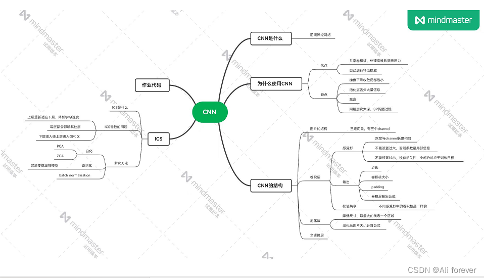
本文介绍了CNN卷积神经网络，希望大家能从中获取到想要的东西，下面附上一张思维导图帮助记忆。

本文来自互联网用户投稿，文章观点仅代表作者本人，不代表本站立场，不承担相关法律责任。如若转载，请注明出处。 如若内容造成侵权/违法违规/事实不符，请点击【内容举报】进行投诉反馈！