SLAM练习题(十一)—— G2O实战
SLAM 学习笔记
写在前面的话:
算是一点小小的感悟吧(* ̄︶ ̄)
估计位姿的方法有线性方法和非线性方法,线性方法就是特征点法中的2D-2D的对极约束,3D-2D的PnP问题。非线性方法有BA优化,它将位姿的估计问题转换成了一个误差关于优化量的最小二乘极值问题,它通过雅克比矩阵指导迭代方向,获得最优的位姿。需要注意的是g2o是一个图优化库,是一个非线性优化库,在使用线性方式求位姿的时候用不到这个库,一般是在使用线性方法(对极约束,PnP……)获得一个误差的估计值后,再用g2o构建图优化问题,设置顶点和边,对位姿进行优化。
但是如果不先求得一个位姿的估计值,直接使用g20构建图优化,将位姿的初始值设为0(或随便设一个初值),进行优化,这样也是可以估计出位姿的,但是迭代次数肯定比先得到一个粗略的位姿再优化要多的多,而且迭代次数与初始值的选取也有很大关系。
文章目录
- 特征点法BA优化
- 分析
- 代码实现
- 雅克比矩阵
- 直接法BA优化
- 分析
- 代码实现
- 讨论
- 双线性插值
- 鲁棒核函数huber
- 雅克比矩阵
特征点法BA优化
分析
以下题目来自计算机视觉life从零开始一起学习SLAM系列
题目: 给定一组世界坐标系下的3D点(p3d.txt)以及它在相机中对应的坐标(p2d.txt),以及相机的内参矩阵。使用
bundle adjustment 方法(g2o库实现)来估计相机的位姿T。初始位姿T为单位矩阵。
(其实就是对3D-2D使用PnP方法得到位姿后,用g2o对该位姿进行优化。)
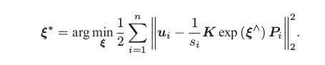
重投影误差:
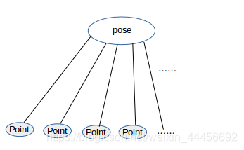
图优化模型:
代码实现
#include (); // 第2步:创建BlockSolver。并用上面定义的线性求解器初始化// Block* solver_ptr = new Block ( std::unique_ptr(linearSolver) ); // 第3步:创建总求解器solver。并从GN, LM, DogLeg 中选一个,再用上述块求解器BlockSolver初始化// g2o::OptimizationAlgorithmLevenberg* solver = new g2o::OptimizationAlgorithmLevenberg ( std::unique_ptr(solver_ptr) ); // 第4步:创建稀疏优化器// g2o::SparseOptimizer optimizer;// optimizer.setAlgorithm ( solver );// old g2o versiontypedef g2o::BlockSolver<g2o::BlockSolverTraits<6,3>> Block; //pose维度为6 landmark 维度为3Block::LinearSolverType* linearSolver = new g2o::LinearSolverCSparse<Block::PoseMatrixType>(); // 线性求解方程器Block* solver_ptr = new Block(linearSolver); // 矩阵求解器g2o::OptimizationAlgorithmLevenberg* solver = new g2o::OptimizationAlgorithmLevenberg(solver_ptr);g2o::SparseOptimizer optimizer;optimizer.setAlgorithm(solver);// 第5步:定义图的顶点和边。并添加到SparseOptimizer中// ----------------------开始你的代码:设置并添加顶点,初始位姿为单位矩阵g2o::VertexSE3Expmap* pose = new g2o::VertexSE3Expmap(); // camera posepose->setId(0);pose->setEstimate(g2o::SE3Quat(Eigen::Matrix3d::Identity(), Eigen::Vector3d::Zero()));optimizer.addVertex(pose);int index =1;for (const Point3f p:points_3d) // 设置空间点 顶点{g2o::VertexSBAPointXYZ* point = new g2o::VertexSBAPointXYZ();point->setId(index++);point->setEstimate(Eigen::Vector3d(p.x,p.y,p.z));point->setMarginalized(true); // 空间点必须要边缘化,以进行加速optimizer.addVertex(point);}// ----------------------结束你的代码// 设置相机内参g2o::CameraParameters* camera = new g2o::CameraParameters (K.at<double> ( 0,0 ), Eigen::Vector2d ( K.at<double> ( 0,2 ), K.at<double> ( 1,2 ) ), 0);camera->setId ( 0 ); // 相机参数 的索引为0optimizer.addParameter ( camera ); // 设置边index = 1; // 边的id是从1开始的 因为空间点顶点的索引是从1 开始的,方便下面的索引for ( const Point2f p:points_2d ){g2o::EdgeProjectXYZ2UV* edge = new g2o::EdgeProjectXYZ2UV();edge->setId ( index );edge->setVertex ( 0, dynamic_cast<g2o::VertexSBAPointXYZ*> ( optimizer.vertex ( index ) ) ); // 第一个顶点: 空间点edge->setVertex ( 1, pose ); // 第二个顶点:位姿edge->setMeasurement ( Eigen::Vector2d ( p.x, p.y ) ); //设置观测值edge->setParameterId ( 0,0 ); // 相机的参数edge->setInformation ( Eigen::Matrix2d::Identity() ); // 信息矩阵optimizer.addEdge ( edge );index++;}// 第6步:设置优化参数,开始执行优化optimizer.setVerbose ( true ); // 输出优化信息,包括迭代次数,cost time, 误差等等optimizer.initializeOptimization();optimizer.optimize ( 100 );// 输出优化结果cout<<endl<<"after optimization:"<<endl;cout<<"T="<<endl<<Eigen::Isometry3d ( pose->estimate() ).matrix() <<endl;
}
这里只考虑了一个位姿。
这是一个最小化重投影问题,使用了g2o 预定好的顶点和边,所以就不用自己再定义了
附CMakeLists.txt:
cmake_minimum_required( VERSION 2.8 )
project( BA )# 添加c++ 11标准支持
set( CMAKE_CXX_FLAGS "-std=c++11" )find_package( OpenCV REQUIRED )# 添加g2o的依赖
# 因为g2o不是常用库,要添加它的findg2o.cmake文件
#set( G2O_ROOT /usr/local/include/g2o )
LIST( APPEND CMAKE_MODULE_PATH ${PROJECT_SOURCE_DIR}/cmake_modules )
find_package( G2O REQUIRED )
find_package( CSparse REQUIRED )# 添加头文件
include_directories( "/usr/include/eigen3"${OpenCV_INCLUDE_DIRS}${G2O_INCLUDE_DIRS}${CSPARSE_INCLUDE_DIR})add_executable( BA BA-3Dto2D.cpp )target_link_libraries( BA${OpenCV_LIBS}${CSPARSE_LIBRARY}g2o_core g2o_stuff g2o_types_sba g2o_csparse_extension)
雅克比矩阵
参考十四讲194页的推导过程:
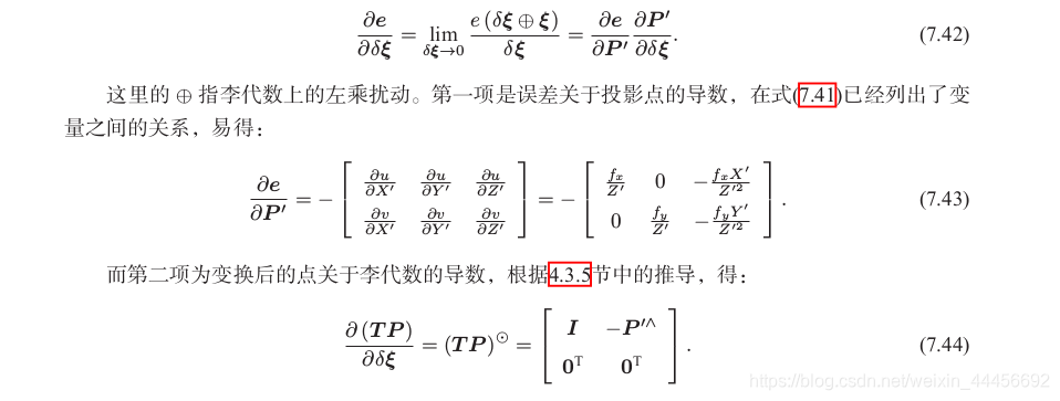
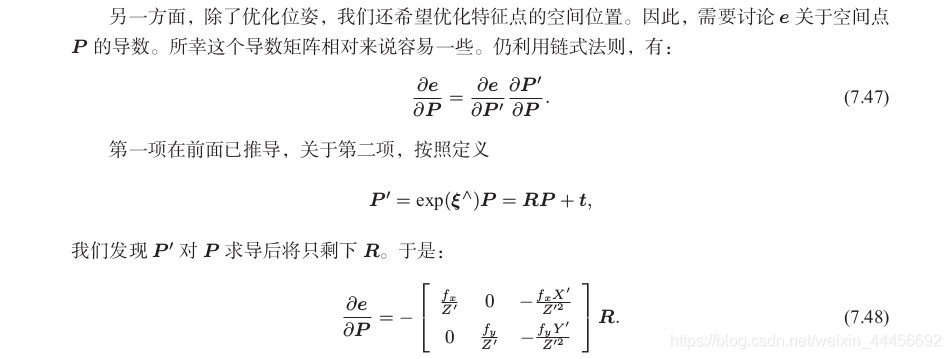
误差相对于空间点P的导数:
稍有差别的是,g2o相机里用f统一描述fx,fy,并且李代数定义顺序不同(g2o是旋转在前,平移在后,书中是平移在前,旋转在后),所以矩阵前三列和后三列与书中的定义是相反的,此外都一致。
直接法BA优化
分析
题目: 用直接法Bundle Adjustment 估计相机位姿。
链接:https://pan.baidu.com/s/105a9WYr0pPOd691leyanjA 提取码:bjzi
知识点: g2o的边
直接法参考14讲上的介绍,主要是灰度不变原则,在这里我们使用一个4*4的窗口内像素的灰度值的误差构建优化目标函数。优化变量为位姿T,三维点P_i,误差为像素点的误差16×1;

代码实现
这次考虑了三个位姿,n个空间点。
g2o本身没有计算光度误差的边,我们需要自己定义。
/***************************** 题目:用直接法Bundle Adjustment 估计相机位姿,已经给定3张图,poses.txt,points.txt文件。** 本程序学习目标:* 熟悉g2o库顶点和边的定义。* * 本代码框架来自高翔,有改动* 公众号:计算机视觉life。发布于公众号旗下知识星球:从零开始学习SLAM* 时间:2019.03
****************************/#include (); // 第2步:创建BlockSolver。并用上面定义的线性求解器初始化// Block* solver_ptr = new Block ( std::unique_ptr(linearSolver) ); // 第3步:创建总求解器solver。并从GN, LM, DogLeg 中选一个,再用上述块求解器BlockSolver初始化// g2o::OptimizationAlgorithmLevenberg* solver = new g2o::OptimizationAlgorithmLevenberg ( std::unique_ptr(solver_ptr) ); // 第4步:创建稀疏优化器// g2o::SparseOptimizer optimizer;// optimizer.setAlgorithm ( solver );// old g2o versiontypedef g2o::BlockSolver< g2o::BlockSolverTraits<6,3> > Block; // pose 维度为 6, landmark 维度为 3Block::LinearSolverType* linearSolver = new g2o::LinearSolverDense<Block::PoseMatrixType>(); // 线性方程求解器Block* solver_ptr = new Block ( linearSolver ); // 矩阵块求解器g2o::OptimizationAlgorithmLevenberg* solver = new g2o::OptimizationAlgorithmLevenberg ( solver_ptr );g2o::SparseOptimizer optimizer;optimizer.setAlgorithm ( solver );// 第5步:添加顶点和边// ---------------- 开始你的代码 ----------------------//// 参考十四讲中直接法BA部分for (int i = 0; i < points.size(); i++){VertexSBAPointXYZ* vertexPw = new VertexSBAPointXYZ();vertexPw->setId(i);vertexPw->setEstimate(points[i]);vertexPw->setMarginalized(true);optimizer.addVertex(vertexPw);}for (int i = 0; i < poses.size(); i++){VertexSophus* vertexTcw = new VertexSophus();vertexTcw->setId(i+points.size());vertexTcw->setEstimate(poses[i]);optimizer.addVertex(vertexTcw);}for (int i = 0; i < poses.size(); i++){for (int j = 0; j < points.size(); j++){ // color里面存的是第j个点周围4*4=16个像素点的灰度值的指针EdgeDirectProjection* edge = new EdgeDirectProjection(color[j], images[i]);edge->setVertex(0, dynamic_cast<VertexSBAPointXYZ*>(optimizer.vertex(j)));edge->setVertex(1, dynamic_cast<VertexSophus*>(optimizer.vertex(i+points.size())));edge->setInformation(Matrix<double,16,16>::Identity());RobustKernelHuber* rk = new RobustKernelHuber; // 鲁棒核函数rk->setDelta(1.0);edge->setRobustKernel(rk);optimizer.addEdge(edge);}}// ---------------- 结束你的代码 ----------------------//// 第6步:执行优化optimizer.initializeOptimization(0);optimizer.optimize(200);// 从optimizer中获取结果for(int c = 0; c < poses.size(); c++)for(int p = 0; p < points.size(); p++) {Vector3d Pw = dynamic_cast<VertexSBAPointXYZ*>(optimizer.vertex(p))->estimate();points[p] = Pw;SE3 Tcw = dynamic_cast<VertexSophus*>(optimizer.vertex(c + points.size()))->estimate();poses[c] = Tcw;}// plot the optimized points and posesDraw(poses, points);// delete color datafor (auto &c: color) delete[] c;return 0;
}// 画图函数,无需关注
void Draw(const VecSE3 &poses, const VecVec3d &points) {if (poses.empty() || points.empty()) {cerr << "parameter is empty!" << endl;return;}cout<<"Draw poses: "<<poses.size()<<", points: "<<points.size()<<endl;// create pangolin window and plot the trajectorypangolin::CreateWindowAndBind("Trajectory Viewer", 1024, 768);glEnable(GL_DEPTH_TEST);glEnable(GL_BLEND);glBlendFunc(GL_SRC_ALPHA, GL_ONE_MINUS_SRC_ALPHA);pangolin::OpenGlRenderState s_cam(pangolin::ProjectionMatrix(1024, 768, 500, 500, 512, 389, 0.1, 1000),pangolin::ModelViewLookAt(0, -0.1, -1.8, 0, 0, 0, 0.0, -1.0, 0.0));pangolin::View &d_cam = pangolin::CreateDisplay().SetBounds(0.0, 1.0, pangolin::Attach::Pix(175), 1.0, -1024.0f / 768.0f).SetHandler(new pangolin::Handler3D(s_cam));while (pangolin::ShouldQuit() == false) {glClear(GL_COLOR_BUFFER_BIT | GL_DEPTH_BUFFER_BIT);d_cam.Activate(s_cam);glClearColor(0.0f, 0.0f, 0.0f, 0.0f);// draw posesfloat sz = 0.1;int width = 640, height = 480;for (auto &Tcw: poses) {glPushMatrix();Sophus::Matrix4f m = Tcw.inverse().matrix().cast<float>();glMultMatrixf((GLfloat *) m.data());glColor3f(1, 0, 0);glLineWidth(2);glBegin(GL_LINES);glVertex3f(0, 0, 0);glVertex3f(sz * (0 - cx) / fx, sz * (0 - cy) / fy, sz);glVertex3f(0, 0, 0);glVertex3f(sz * (0 - cx) / fx, sz * (height - 1 - cy) / fy, sz);glVertex3f(0, 0, 0);glVertex3f(sz * (width - 1 - cx) / fx, sz * (height - 1 - cy) / fy, sz);glVertex3f(0, 0, 0);glVertex3f(sz * (width - 1 - cx) / fx, sz * (0 - cy) / fy, sz);glVertex3f(sz * (width - 1 - cx) / fx, sz * (0 - cy) / fy, sz);glVertex3f(sz * (width - 1 - cx) / fx, sz * (height - 1 - cy) / fy, sz);glVertex3f(sz * (width - 1 - cx) / fx, sz * (height - 1 - cy) / fy, sz);glVertex3f(sz * (0 - cx) / fx, sz * (height - 1 - cy) / fy, sz);glVertex3f(sz * (0 - cx) / fx, sz * (height - 1 - cy) / fy, sz);glVertex3f(sz * (0 - cx) / fx, sz * (0 - cy) / fy, sz);glVertex3f(sz * (0 - cx) / fx, sz * (0 - cy) / fy, sz);glVertex3f(sz * (width - 1 - cx) / fx, sz * (0 - cy) / fy, sz);glEnd();glPopMatrix();}// pointsglPointSize(2);glBegin(GL_POINTS);for (size_t i = 0; i < points.size(); i++) {glColor3f(0.0, points[i][2]/4, 1.0-points[i][2]/4);glVertex3d(points[i][0], points[i][1], points[i][2]);}glEnd();pangolin::FinishFrame();usleep(5000); // sleep 5 ms}
}附CMakeLists.txt
cmake_minimum_required( VERSION 2.8 )
project( directBA )# 添加c++ 11标准支持
set( CMAKE_CXX_FLAGS "-std=c++11 -O3" )
list( APPEND CMAKE_MODULE_PATH ${PROJECT_SOURCE_DIR}/cmake_modules )
set(G2O_LIBS g2o_cli g2o_ext_freeglut_minimal g2o_simulator g2o_solver_slam2d_linearg2o_types_icp g2o_types_slam2d g2o_types_sba g2o_types_slam3d g2o_core g2o_interfaceg2o_solver_csparse g2o_solver_structure_only g2o_csparse_extension g2o_opengl_helper g2o_solver_denseg2o_stuff g2o_types_sclam2d g2o_parser g2o_solver_pcg g2o_types_data g2o_types_sim3 cxsparse )
# 添加cmake模块以使用g2o库
list( APPEND CMAKE_MODULE_PATH ${PROJECT_SOURCE_DIR}/cmake_modules )
find_package( G2O REQUIRED)
find_package( Eigen3 REQUIRED)
find_package( OpenCV REQUIRED )beijign
find_package( Sophus REQUIRED )
find_package( Pangolin REQUIRED)# 添加头文件
include_directories( "/usr/include/eigen3" )
include_directories( ${OpenCV_INCLUDE_DIRS} )
include_directories( ${Sophus_INCLUDE_DIRS} )
include_directories( ${Pangolin_INCLUDE_DIRS})
include_directories( ${G2O_INCLUDE_DIRS})add_executable( directBA directBA.cpp )target_link_libraries( directBA ${OpenCV_LIBS} ${G2O_LIBS})
target_link_libraries( directBA ${Sophus_LIBRARIES} )
target_link_libraries( directBA   /home/yan/3rdparty/Sophus/build/libSophus.so )
target_link_libraries( directBA ${Pangolin_LIBRARIES})
讨论
双线性插值
通过双线性差值获得浮点坐标对应插值后的像素值
背景:把空间点point(x,y,z)经过投影计算得到的图像坐标(u,v)(即下面函数的输入参数x,y)不一定是整数,我们需要对该浮点数进行插值处理。
// bilinear interpolation 通过双线性差值获得浮点坐标对应插值后的像素值
inline float GetPixelValue(const cv::Mat &img, float x, float y) {uchar *data = &img.data[int(y) * img.step + int(x)];	// 取得该像素值的data位置 step为Mat中一行所占的字节数float xx = x - floor(x);	// xx 为x的小数部分float yy = y - floor(y);	// yy为y的小数部分。return float((1 - xx) * (1 - yy) * data[0] +xx * (1 - yy) * data[1] +(1 - xx) * yy * data[img.step] +xx * yy * data[img.step + 1]);
}
在图像的仿射变换(图像的放大缩小)中,很多地方需要用到插值运算,常见的插值运算包括最邻近插值,双线性插值,双三次插值,兰索思插值等方法,OpenCV提供了很多方法,其中,双线性插值由于折中的插值效果和运算速度,用的最多。
双线性插值算法:
对于一个目的像素,设置坐标通过反向变换得到的浮点坐标为(i+u,j+v) (其中i、j均为浮点坐标的整数部分,u、v为浮点坐标的小数部分,是取值[0,1)区间的浮点数),则这个像素得值 f(i+u,j+v) 可由原图像中坐标为 (i,j)、(i+1,j)、(i,j+1)、(i+1,j+1)所对应的周围四个像素的值决定,即:f(i+u,j+v) = (1-u)(1-v)f(i,j) + (1-u)vf(i,j+1) + u(1-v)f(i+1,j) + uvf(i+1,j+1),其中f(i,j)表示源图像(i,j)处的的像素值,以此类推。
对应于程序里面:
data[0]为f(i,j),data[1]为f(i,j+1),data[img.step]为f(i+1,j), data[img.step+1]为f(i+1,j+1)
具体推导过程可参考:图像处理之双线性插值法
鲁棒核函数huber
参考维基百科:huber

当误差e大于某个阈值后,函数增长由二次形式变成了一次形式,相当于限制了梯度的最大值,同时Huber核函数又是光滑的,可以很方便的求导。参考Slam十四讲255页。
雅克比矩阵
推导过程参考14讲194页。
首先是光度误差关于位姿扰动量的导数,这里的q相当于特征点法中的P’,表示相机坐标系下的点。
。
J = − ∂ I 2 ∂ u ∂ u ∂ q ∂ q ∂ δ ξ = − ∂ I 2 ∂ u ∂ u ∂ δ ξ \large J=-\frac{\partial{I_2}}{\partial{u}}\frac{\partial{u}}{\partial{q}}\frac{\partial{q}}{\partial{\delta\xi}}=-\frac{\partial{I_2}}{\partial{u}}\frac{\partial{u}}{\partial{\delta\xi}} J=−∂u∂I2∂q∂u∂δξ∂q=−∂u∂I2∂δξ∂u
- ∂ I 2 ∂ u \LARGE \frac{\partial{I_2}}{\partial{u}} ∂u∂I2是u处的像素梯度
在上面 的代码中,使用了中值定理来计算梯度:
J_I_Puv(0,0) = (GetPixelValue(targetImg,u+i+1,v+j) - GetPixelValue(targetImg,u+i-1,v+j))/2;J_I_Puv(0,1) = (GetPixelValue(targetImg,u+i,v+j+1) - GetPixelValue(targetImg,u+i,v+j-1))/2;
也就是利用u处的前一个点和后一个点的像素均值来代替u处的像素梯度。
- ∂ u ∂ q \LARGE \frac{\partial{u}}{\partial{q}} ∂q∂u为投影方程关于相机坐标系下的三维点的导数
也就是像素坐标 [ u v ] \begin{bmatrix}u \\v \end{bmatrix} [uv]关于相机坐标系下三维点q [ X ’ Y ′ Z ′ ] \begin{bmatrix} X’&Y'&Z'\end{bmatrix} [X’Y′Z′]的导数:
∂ u ∂ q = [ f x Z ′ 0 − f x X ′ Z ′ 2 0 f y Z ′ − f y Y ′ Z ′ 2 ] \large \frac{\partial u}{\partial q}=\begin{bmatrix}\frac{f_x}{Z'}&0&-\frac{f_xX'}{Z'^2}\\ 0&\frac{f_y}{Z'}&-\frac{f_yY'}{Z'^2}\end{bmatrix} ∂q∂u=⎣⎡Z′fx00Z′fy−Z′2fxX′−Z′2fyY′⎦⎤
- ∂ q ∂ δ ξ \LARGE \frac{\partial q}{\partial \delta\xi} ∂δξ∂q为变换后的三维点(相机坐标系下的点)对位姿扰动量的导数。
在求左乘扰动的时候,已经证明:
∂ q ∂ δ ξ = [ I , − q ∧ ] \large \frac{\partial q}{\partial \delta \xi}=\begin{bmatrix}I,&-q^{\wedge}\end{bmatrix} ∂δξ∂q=[I,−q∧]
其中
q ∧ = [ 0 − Z ′ Y ′ Z ′ 0 − X ′ − Y ′ X ′ 0 ] \large q^{\wedge}=\begin{bmatrix}0&-Z'&Y'\\ Z'&0&-X'\\ -Y'&X'&0 \end{bmatrix} q∧=⎣⎢⎡0Z′−Y′−Z′0X′Y′−X′0⎦⎥⎤
后两项只与三维点P有关,而与图像无关,经常将这两项合并在一起:
∂ u ∂ δ ξ = [ f x Z ′ 0 − f x X ′ Z ′ 2 − f x X ′ Y ′ Z ′ 2 f x + f x X ′ 2 Z ′ 2 − f x Y ′ Z ′ 0 f y Z ′ − f y Y ′ Z ′ 2 − f y − f y Y ′ 2 Z ′ 2 f y X ′ Y ′ Z ′ 2 f y X ′ Z ′ ] \large \frac{\partial{u}}{\partial{\delta\xi}}=\begin{bmatrix}\frac{f_x}{Z'}&0&-\frac{f_xX'}{Z'^2} &-\frac{f_xX'Y'}{Z'^2}&f_x+\frac{f_xX'^2}{Z'^2}&-\frac{f_xY'}{Z'}\\ 0&\frac{f_y}{Z'}&-\frac{f_yY'}{Z'^2}&-f_y-\frac{f_yY'^2}{Z'^2}&\frac{f_yX'Y'}{Z'^2}&\frac{f_yX'}{Z'}\end{bmatrix} ∂δξ∂u=⎣⎡Z′fx00Z′fy−Z′2fxX′−Z′2fyY′−Z′2fxX′Y′−fy−Z′2fyY′2fx+Z′2fxX′2Z′2fyX′Y′−Z′fxY′Z′fyX′⎦⎤
所以光度误差相对于李代数的雅克比矩阵为:
J = − ∂ I 2 ∂ u ∂ u ∂ δ ξ \large J=-\frac{\partial{I_2}}{\partial{u}}\frac{\partial{u}}{\partial{\delta\xi}} J=−∂u∂I2∂δξ∂u
光度误差关于空间点的导数:
和特征点法中的求法差不多:
∂ I ∂ P = ∂ I ∂ u ∂ u ∂ q ∂ q ∂ P \large \frac{\partial I}{\partial P}=\frac{\partial I}{\partial u}\frac{\partial u}{\partial q}\frac{\partial q}{\partial P} ∂P∂I=∂u∂I∂q∂u∂P∂q
前两项分别是像素梯度和投影坐标关于Pc的偏导数,第三项是Pc关于Pw的偏导数,又因为 q = e x p ( ξ ∧ ) P = R P + t q=exp(\xi^{\wedge})P=RP+t q=exp(ξ∧)P=RP+t,所以q对P的求导后只剩下R,于是:
∂ I ∂ P = ∂ I ∂ u ∂ u ∂ q R \large \frac{\partial I}{\partial P}=\frac{\partial I}{\partial u}\frac{\partial u}{\partial q}R ∂P∂I=∂u∂I∂q∂uR
在代码中为:
_jacobianOplusXi.block<1,3>(num,0) = -J_I_Puv * J_Puv_Pc * vertexTcw->estimate().rotation_matrix();_jacobianOplusXj.block<1,6>(num,0) = -J_I_Puv * J_Puv_Pc * J_Pc_kesi;
_jacobianOplusXi为光度误差对空间点的导数,里面存放16行1*3的矩阵。
_jacobianOplusXj光度误差对位姿(扰动量)的导数,里面存放16行1*6的矩阵。
参考:
视觉SLAM14讲
从零开始一起学习SLAM | 掌握g2o顶点编程套路
从零开始一起学习SLAM | 掌握g2o边的代码套路
本文来自互联网用户投稿,文章观点仅代表作者本人,不代表本站立场,不承担相关法律责任。如若转载,请注明出处。 如若内容造成侵权/违法违规/事实不符,请点击【内容举报】进行投诉反馈!