样本不均衡案例及解决办法

• 一、样本不均衡问题描述与解决办法
• • 1、样本不均衡问题描述
  • 2、常用解决办法
• 二、实例分析
• • 1、数据集来源与介绍
  • 2、数据集导入与初探
  • 3、数据清洗与预处理
  • • 3.1 缺失值处理
    • 3.2 特征筛选
    • 3.3 数据转换
  • 4、预测结果对比
  • • 4.1 未处理样本不均衡问题数据集模型
    • 4.2 采用SMOTE处理样本不均衡问题数据集模型

一、样本不均衡问题描述与解决办法

1、样本不均衡问题描述

问题描述：
先举一个“恐怖”的例子，直观的感受一下样本不平衡问题：

你根据1000个正样本和1000个负样本正确训练出了一个正确率90%召回率90%的分类器，且通过实验验证没有欠采样过采样的问题哦。完美的样本，完美的模型，破费，你心里暗自得意。然后模型上线，正式预测每天的未知样本~。

开始一切都很美好，正确率召回率都很好。直到有一天，数据发生了一点变化，还是原来的数据类型和特征，只是每天新数据中正负样本变成了100个正样本，10000个负样本。注意，先前正确率90%的另一种表达是负样本有10%的概率被误检为正样本。好了，模型不变，现在误检的负样本数是100000.1=1000个，正样本被检出1000.9（召回）=90个，好了，这个时候召回率不变仍为90%，但是新的正确率=90/(1000+90)=8.26% 。震惊吗！？恐怖吗！？

结论： 同一个模型仅仅是改变了验证集的正负样本比例，模型已经从可用退化成不可用了！！样本不平衡问题可怕就可怕在这，往往你的模型参数，训练，数据，特征都是对的！能做的都做了，但你的正确率就是上不去！！绝望吧。。。。。。

在现实中有很多类别不均衡问题，它是常见的，并且也是合理的，符合人们期望的。如，在欺诈交易识别中，属于欺诈交易的应该是很少部分，即绝大部分交易是正常的，只有极少部分的交易属于欺诈交易。这就是一个正常的类别不均衡问题。又如，在客户流失的数据集中，绝大部分的客户是会继续享受其服务的（非流失对象），只有极少数部分的客户不会再继续享受其服务（流失对象）。一般而已，如果类别不平衡比例超过4:1，那么其分类器会大大地因为数据不平衡性而无法满足分类要求的。因此在构建分类模型之前，需要对分类不均衡性问题进行处理。
  
  在前面，我们使用正确率这个指标来评价分类质量，可以看出，在类别不均衡时，正确率这个评价指标并不能work。因为分类器将所有的样本都分类到大类下面时，该指标值仍然会很高。即，该分类器偏向了大类这个类别的数据。

2、常用解决办法

样本类别不均衡将导致样本量少的分类所包含的特征过少，并很难从中提取规律；即使得到分类模型，也容易产生过度依赖与有限的数据样本而导致过拟合问题，当模型应用到新的数据上时，模型的准确性会很差。
常用的解决办法包括以下几种：

• SMOTE(Synthetic Minority Over-sampling Technique)过采样小样本（扩充小类，产生新数据）
  即该算法构造的数据是新样本，原数据集中不存在的。该基于距离度量选择小类别下两个或者更多的相似样本，然后选择其中一个样本，并随机选择一定数量的邻居样本对选择的那个样本的一个属性增加噪声，每次处理一个属性。这样就构造了更多的新生数据。（优点是相当于合理地对小样本的分类平面进行的一定程度的外扩；也相当于对小类错分进行加权惩罚（解释见3））

• 欠采样大样本（压缩大类，产生新数据）
  设小类中有N个样本。将大类聚类成N个簇，然后使用每个簇的中心组成大类中的N个样本，加上小类中所有的样本进行训练。（优点是保留了大类在特征空间的分布特性，又降低了大类数据的数目）

• 对小类错分进行加权惩罚
  对分类器的小类样本数据增加权值，降低大类样本的权值（这种方法其实是产生了新的数据分布，即产生了新的数据集，译者注），从而使得分类器将重点集中在小类样本身上。一个具体做法就是，在训练分类器时，若分类器将小类样本分错时额外增加分类器一个小类样本分错代价，这个额外的代价可以使得分类器更加“关心”小类样本。如penalized-SVM和penalized-LDA算法。
  对小样本进行过采样（例如含L倍的重复数据），其实在计算小样本错分cost functions时会累加L倍的惩罚分数。

二、实例分析

1、数据集来源与介绍

• 数据集来自UCI机器学习库：数据集链接
• 数据集为葡萄牙银行的电话营销数据， 分类目标是预测客户是否会开设到定期存款账户（预测值y）。包含银行客户的个人属性特征、社会与经济属性特征等字段，共41189条记录，每个字段的详细描述如下：
• bank client data:
  1 - age (numeric)
  2 - job : type of job (categorical: ‘admin.’,‘blue-collar’,‘entrepreneur’,‘housemaid’,‘management’,‘retired’,‘self-employed’,‘services’,‘student’,‘technician’,‘unemployed’,‘unknown’)
  3 - marital : marital status (categorical: ‘divorced’,‘married’,‘single’,‘unknown’; note: ‘divorced’ means divorced or widowed)
  4 - education (categorical: ‘basic.4y’,‘basic.6y’,‘basic.9y’,‘high.school’,‘illiterate’,‘professional.course’,‘university.degree’,‘unknown’)
  5 - default: has credit in default? (categorical: ‘no’,‘yes’,‘unknown’)
  6 - housing: has housing loan? (categorical: ‘no’,‘yes’,‘unknown’)
  7 - loan: has personal loan? (categorical: ‘no’,‘yes’,‘unknown’)
• related with the last contact of the current campaign:
  8 - contact: contact communication type (categorical: ‘cellular’,‘telephone’)
  9 - month: last contact month of year (categorical: ‘jan’, ‘feb’, ‘mar’, …, ‘nov’, ‘dec’)
  10 - day_of_week: last contact day of the week (categorical: ‘mon’,‘tue’,‘wed’,‘thu’,‘fri’)
  11 - duration: last contact duration, in seconds (numeric). Important note: this attribute highly affects the output target (e.g., if duration=0 then y=‘no’). Yet, the duration is not known before a call is performed. Also, after the end of the call y is obviously known. Thus, this input should only be included for benchmark purposes and should be discarded if the intention is to have a realistic predictive model.
• other attributes:
  12 - campaign: number of contacts performed during this campaign and for this client (numeric, includes last contact)
  13 - pdays: number of days that passed by after the client was last contacted from a previous campaign (numeric; * 999 means client was not previously contacted)
  14 - previous: number of contacts performed before this campaign and for this client (numeric)
  15 - poutcome: outcome of the previous marketing campaign (categorical: ‘failure’,‘nonexistent’,‘success’)
• social and economic context attributes
  16 - emp.var.rate: employment variation rate - quarterly indicator (numeric)
  17 - cons.price.idx: consumer price index - monthly indicator (numeric)
  18 - cons.conf.idx: consumer confidence index - monthly indicator (numeric)
  19 - euribor3m: euribor 3 month rate - daily indicator (numeric)
  20 - nr.employed: number of employees - quarterly indicator (numeric)
• Output variable (desired target):
  21 - y - has the client subscribed a term deposit? (binary: ‘yes’,‘no’)

2、数据集导入与初探

导入所需模块：

import pandas as pd
import numpy as np
# from tqdm import tqdm 
# from glob import glob 
import datetime
import matplotlib.pyplot as plt
import matplotlib
import seaborn as sns
matplotlib.get_cachedir() # 清除一下matplotlib的cache
from matplotlib.font_manager import FontProperties
myfont=FontProperties(fname=r'C:\Windows\Fonts\simhei.ttf',size=14) # 设置matplotlib画图支持中文
sns.set(font=myfont.get_name()) # 设置sns画图支持中文
matplotlib.rcParams['axes.unicode_minus'] = False # 解决matplotlib画图符号变方块的现象
%matplotlib inline
import sys,warnings
sys._enablelegacywindowsfsencoding()
warnings.filterwarnings('ignore') 
from sklearn.model_selection import train_test_split
from sklearn.linear_model import LogisticRegression
from sklearn import preprocessing

导入数据集：

# 导入数据集
data = pd.read_csv(r"C:\Users\Administrator\Desktop\machinelearningdemo\greedy_school\LogisticRegression\banking.csv")
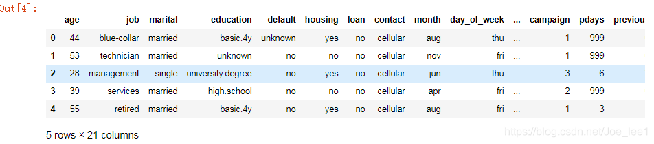
data.head()
plt.figure(figsize=(8,8))
data['y'].value_counts().plot(kind='pie', autopct='%1.1f%%', title='是否开设定期存款账户')

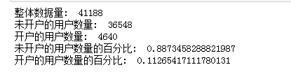
• 未开户的百分比: 88.7% 开户的百分比: 11.3% 样本类别之间比例接近8:1，属于不均衡样本案例。
• 数据集共41188 rows * 21 columns，数据无缺失值，包含job、marital、education、default、housing、loan、contact、month、day_of_week、poutcome类别型字段。

# 数据初探
data.groupby(["y"]).mean()

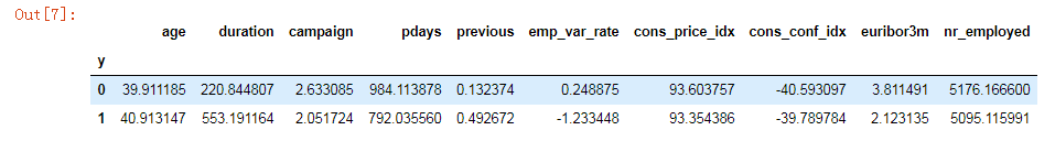
• 购买定期存款的客户的平均年龄高于未购买定期存款的客户的平均年龄。
• 购买定期存款的客户的 pdays（自上次联系客户以来的日子）较低。 pdays越低，最后一次通话的记忆越好，因此销售的机会就越大。
• 此外，购买定期存款的客户的销售通话次数较低。
  在数据预处理时，可采取可视化以及独立性分析手段，以更详细地了解我们的数据，并找出与目标变量（是否开户y）强相关的特征。

3、数据清洗与预处理

逻辑回归模型对变量的要求：

• 变量间不存在较强的线性相关性和多重共线性；
• 变量具有显著性；
• 变量具有合理的业务含义。

3.1 缺失值处理

数据集质量较好，不存在缺失值，因此不需要对缺失值进行处理。

3.2 特征筛选

• step 1：去掉特征中只有一种属性的列

# 在原始数据中的特征值或者属性里都是一样的，对于分类模型的预测是没有用的
# 某列特征都是n n n  NaN  n n ,有缺失的，唯一的属性就有2个，用pandas空值给去掉orig_columns = data.columns  #展现出所有的列
drop_columns = []  #初始化空值
for col in orig_columns:# 使用dropna()先删除空值，再去重算唯一的属性col_series = data[col].dropna().unique()  #去重唯一的属性if len(col_series) == 1:  #如果该特征的属性只有一个属性，就给过滤掉该特征drop_columns.append(col)data = data.drop(drop_columns, axis=1)
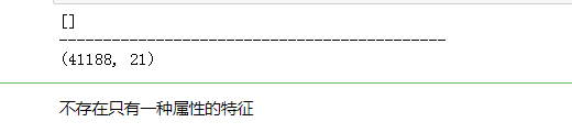
print(drop_columns)
print("--------------------------------------------")
print(data.shape)

• step 2：基于因素分析与独立性分析，来筛选出对目标变量显著的因素以及过滤强相关的自变量

# 单因素分析主要采取可视化手段
y_col = "y"
# 类别型变量：cat_cols = ["job", "marital", "education", "default", "housing", "loan", "contact", "month", "day_of_week", "poutcome"]
plt_cols = ["job", "marital", "education", "default"]
plt.figure(figsize=[15,10])
i = 1
for col in plt_cols:ax = plt.subplot(220+i)sns.barplot(col, y_col, data=data)ax.set_xticklabels(ax.get_xticklabels(), rotation=30)i+=1

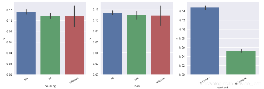
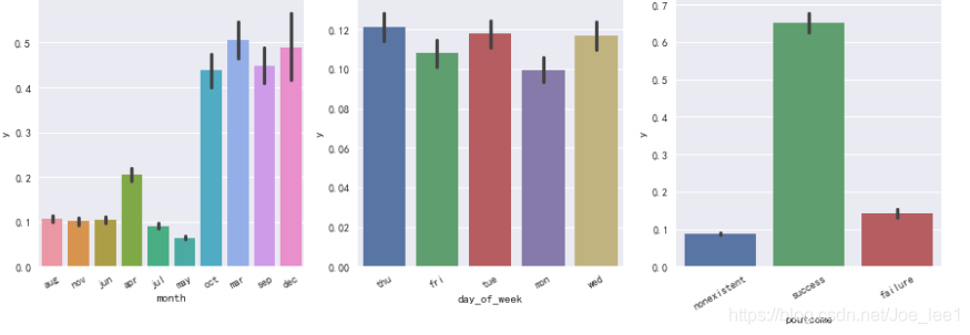
结果显示：housing\loan\day_of_week三个变量与目标变量之间相关性低，似乎不是很好的预测因素。

# 数值型变量：num_cols = ["age", "duration", "campaign", "pdays", "previous", "emp_var_rate", "cons_price_idx", "cons_conf_idx", "euribor3m", "nr_employed"]plt_cols = ["age", "duration", "campaign", "pdays"]
no_col,yes_col = "green","red"
plt.figure(figsize=[15,6])
i = 1
for col in plt_cols:ax = plt.subplot(220+i)sns.distplot(data[data[y_col]==0][col].dropna().values, kde=True, bins=50, color=no_col)sns.distplot(data[data[y_col]==1][col].dropna().values, kde=True, bins=50, color=yes_col,axlabel=col)ax.set_xticklabels(ax.get_xticklabels(), rotation=30)i+=1

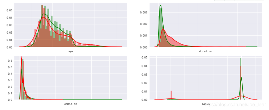
结果显示，年轻与年长的更倾向于在银行开定期存款账户；最近一次电话推销沟通时间长的更倾向于开户。

# 数值型变量：num_cols = ["age", "duration", "campaign", "pdays", "previous", "emp_var_rate", "cons_price_idx", "cons_conf_idx", "euribor3m", "nr_employed"]plt_cols = ["previous", "emp_var_rate", "cons_price_idx", "cons_conf_idx", "euribor3m", "nr_employed"]
no_col,yes_col = "green","red"
plt.figure(figsize=[15,6])
i = 1
for col in plt_cols:ax = plt.subplot(230+i)sns.distplot(data[data[y_col]==0][col].dropna().values, kde=True, bins=50, color=no_col)sns.distplot(data[data[y_col]==1][col].dropna().values, kde=True, bins=50, color=yes_col,axlabel=col)ax.set_xticklabels(ax.get_xticklabels(), rotation=30)i+=1

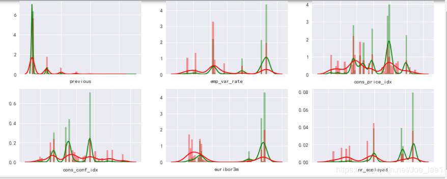
结果显示，欧元每三月利率越低时倾向于开户；季度职工人数越低越倾向于开户。

# 多因素分析：分为类别型-类别型，类别型-数值型，数值型-数值型
# a、类别型-类别型示例
# cat_cols = ["job", "marital", "education", "default", "housing", "loan", "contact", "month", "day_of_week", "poutcome"]
# housing\loan\day_of_week
# job*housing
grid = sns.FacetGrid(data, col="housing", size=5, aspect=1.6) 
grid.map(sns.barplot, "job", y_col, alpha=.5, ci=None)
grid.set_xticklabels(rotation=30)
grid.add_legend()

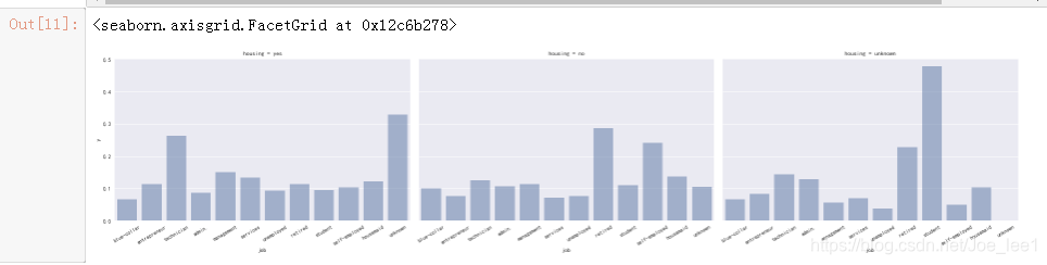
退休没有房贷的更倾向于开户；有房贷的技术员更倾向于开户…

# marital * education
data['education']=np.where(data['education'] =='basic.9y', 'Basic', data['education'])
data['education']=np.where(data['education'] =='basic.6y', 'Basic', data['education'])
data['education']=np.where(data['education'] =='basic.4y', 'Basic', data['education']) # 压缩教育程度类别grid = sns.FacetGrid(data, col="marital", size=5, aspect=1.6) 
grid.map(sns.barplot, "education", y_col, alpha=.5, ci=None)
grid.set_xticklabels(rotation=30)
grid.add_legend()

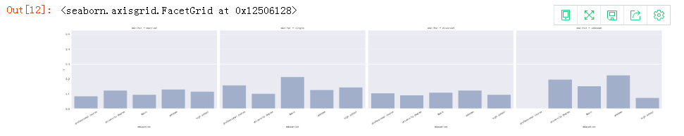
仅受基础教育的单身人士更倾向于开户，其余类别开户的概率相差不大。

# 类别型—数值型
# age * job
grid = sns.FacetGrid(data, col=y_col, size=5, aspect=1.6)
grid.map(sns.pointplot, 'job', 'age', palette='deep')
grid.set_xticklabels(rotation=30)
grid.add_legend()

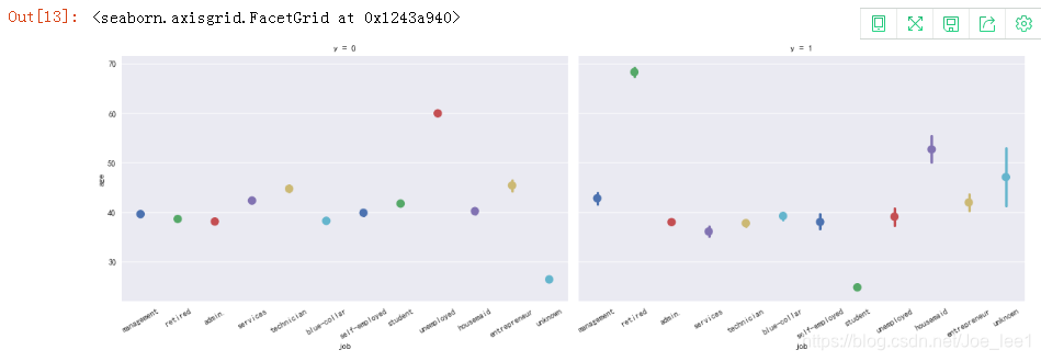
相对年老的退休人员更倾向于开户；相对年老的未受雇人员更不易于开户。

# 数值型-数值型 独立性分析，绘制矩阵热图
plt.figure(figsize=(14,12))
foo = sns.heatmap(data[num_cols].corr(), vmax=0.6, square=True, annot=True)

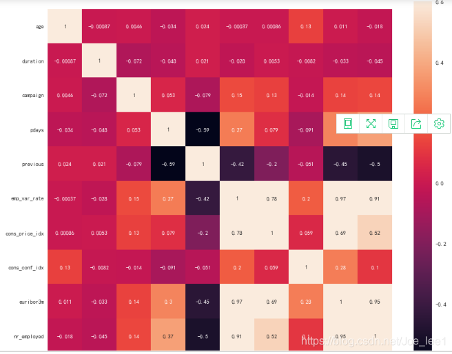
其中emp_var_rate\euribor3m与其余变量之间存在较强的相关性，可在建模时过滤掉该特征。 基于因素分析与独立性分析，筛选出变量如下：

num_cols = [“age”, “duration”, “campaign”, “pdays”, “previous”, “cons_price_idx”, “cons_conf_idx”, “nr_employed”]
cat_cols = [“job”, “marital”, “education”, “default”, “contact”, “month”, “poutcome”]

3.3 数据转换

由于sk-learn库不接受字符型的数据，所以还需将筛选出的特征中字符型的数据进行转换。

cat_vars=['job','marital','education','default','contact','month','poutcome']
for var in cat_vars:cat_list = pd.get_dummies(data_1[var], prefix=var)data_1 = data_1.join(cat_list)data_final_1 = data_1.drop(cat_vars, axis=1)
data_final_1 = data_final_1.drop(["emp_var_rate", "euribor3m"], axis=1)
data_final_1 = data_final_1.drop(["housing", "loan", "day_of_week"], axis=1)
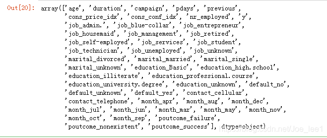
data_final_1.columns.values

4、预测结果对比

4.1 未处理样本不均衡问题数据集模型

• 测试集训练集切分：

from sklearn.model_selection import train_test_split
X = data_final_1.loc[:, data_final_1.columns != 'y']
y = data_final_1.loc[:, data_final_1.columns == 'y']
X_train, X_test, y_train, y_test = train_test_split(X, y, test_size=0.3, random_state=0)
# we can Check the numbers of our data
print("整体数据量: ",len(X))
print("未开户的用户数量: ",len(y[y['y']==0]))
print("开户的用户数量: ",len(y[y['y']==1]))
print("未开户的用户数量的百分比: ",len(y[y['y']==0])/len(X))
print("开户的用户数量的百分比: ",len(y[y['y']==1])/len(X))

• 数据建模与评价：

from sklearn.linear_model import LogisticRegression
from sklearn import metrics
from sklearn.metrics import classification_report
# 创建训练器
lrreg = LogisticRegression()
lrreg.fit(X_train, y_train.values.reshape(-1))
y_pred = lrreg.predict(X_test)
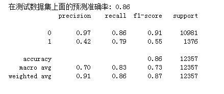
print('在测试数据集上面的预测准确率: {:.2f}'.format(lrreg.score(X_test, y_test)))
print(classification_report(y_test, y_pred))

在测试数据集上面的预测准确率: 0.91。

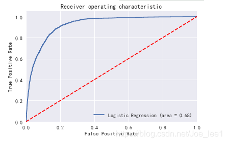
# 绘制ROC曲线
from sklearn.metrics import roc_auc_score
from sklearn.metrics import roc_curve
logit_roc_auc = roc_auc_score(y_test, lrreg.predict(X_test))
fpr, tpr, thresholds = roc_curve(y_test, lrreg.predict_proba(X_test)[:,1])
plt.figure()
plt.plot(fpr, tpr, label='Logistic Regression (area = %0.2f)' % logit_roc_auc)
plt.plot([0, 1], [0, 1],'r--')
plt.xlim([0.0, 1.0])
plt.ylim([0.0, 1.05])
plt.xlabel('False Positive Rate')
plt.ylabel('True Positive Rate')
plt.title('Receiver operating characteristic')
plt.legend(loc="lower right")
plt.savefig('Log_ROC')
plt.show()

4.2 采用SMOTE处理样本不均衡问题数据集模型

注意：在进行数据增广的时候一定要将测试集和验证集单独提前分开，扩张只在训练集上进行，否则会造成在增广的验证集和测试集上进行验证和测试，在实际上线后再真实数据中效果可能会非常的差。

• 测试集训练集切分：

X = data_final_1.loc[:, data_final_1.columns != 'y']
y = data_final_1.loc[:, data_final_1.columns == 'y'].values.ravel()from imblearn.over_sampling import SMOTE
os = SMOTE(random_state=0)
X_train, X_test, y_train, y_test = train_test_split(X, y, test_size=0.3, random_state=0)
columns = X_train.columns
os_data_X,os_data_y=os.fit_sample(X_train, y_train)
os_data_X = pd.DataFrame(data=os_data_X,columns=columns )
os_data_y= pd.DataFrame(data=os_data_y,columns=['y'])
# we can Check the numbers of our data
print("过采样以后的数据量: ",len(os_data_X))
print("未开户的用户数量: ",len(os_data_y[os_data_y['y']==0]))
print("开户的用户数量: ",len(os_data_y[os_data_y['y']==1]))
print("未开户的用户数量的百分比: ",len(os_data_y[os_data_y['y']==0])/len(os_data_X))
print("开户的用户数量的百分比: ",len(os_data_y[os_data_y['y']==1])/len(os_data_X))

• 模型构建与评价：

# 创建训练器
lrreg = LogisticRegression()
lrreg.fit(os_data_X, os_data_y.values.reshape(-1))
y_pred = lrreg.predict(X_test)
print('在测试数据集上面的预测准确率: {:.2f}'.format(lrreg.score(X_test, y_test)))
print(classification_report(y_test, y_pred))

# 绘制roc曲线
logit_roc_auc = roc_auc_score(y_test, lrreg.predict(X_test))
fpr, tpr, thresholds = roc_curve(y_test, lrreg.predict_proba(X_test)[:,1])
plt.figure()
plt.plot(fpr, tpr, label='Logistic Regression (area = %0.2f)' % logit_roc_auc)
plt.plot([0, 1], [0, 1],'r--')
plt.xlim([0.0, 1.0])
plt.ylim([0.0, 1.05])
plt.xlabel('False Positive Rate')
plt.ylabel('True Positive Rate')
plt.title('Receiver operating characteristic')
plt.legend(loc="lower right")
plt.savefig('Log_ROC')
plt.show()

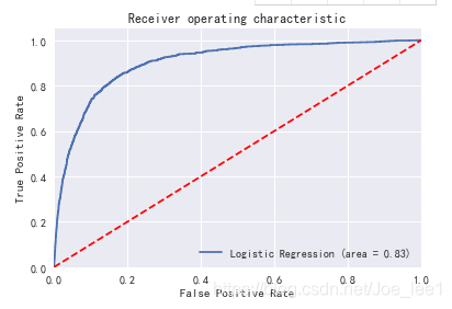
可以从结果中发现，未处理样本不均衡的数据集模型预测结果中正确率高于处理后的模型预测结果，但是其对于小样本类的召回率明显低于处理后的模型预测结果，f1值、AUC值也较低。
参考文献：样本不平衡问题分析与部分解决办法

本文来自互联网用户投稿，文章观点仅代表作者本人，不代表本站立场，不承担相关法律责任。如若转载，请注明出处。 如若内容造成侵权/违法违规/事实不符，请点击【内容举报】进行投诉反馈！