matlab绘制海表面温度、盐度等要素

一般使用nc文件。

下载文件，读取文件，绘制海表面要素图。

数据源：WOA 2018 (noaa.gov)

代码：

clear;
clc;source1 = 'woa18_decav_t00_04.nc';         %读取文件
ncdisp(source1);                           %查阅nc文件信息
boundary = [-180 180 -90 90];              %设置经纬度范围lon      = ncread(source1,'lon');         %查阅经度信息
loncount = length(lon);                   %查阅经度精度（有多少格点）
lat      = ncread(source1,'lat');         %查阅纬度信息
latcount = length(lat);                   %查阅纬度精度（有多少格点）
time     = ncread(source1,'time');        %查阅时间层数信息
ticount  = length(time);                  %查阅时间层数t        = 1;
varname  = 't_an';                        %根据ncdisp显示的变量输入绘图lon_scope  = find(lon >= boundary(1) & lon <= boundary(2));
lat_scope  = find(lat >= boundary(3) & lat <= boundary(4));
lon_number = length(lon_scope);
lat_number = length(lat_scope);start   = [lon_scope(1),lat_scope(1),1,1];             %初始位置
count   = [lon_number,lat_number,ticount,1];           %读取范围
stride1 = [1,1,1,1];                                   %读取步长
sst1    = ncread(source1,varname,start,count,stride1); %读取温度
%sst2   = sst1-273.15;                                 %若数据是开尔文需要转换的话
sst_plot = imrotate(sst1(:,:,t), 90);                  %旋转矩阵，因为matlab是列优先
SST_plot = flipud(sst_plot); 
m_proj('Miller Cylindrical','lat',[boundary(3) boundary(4)],'lon',[boundary(1) boundary(2)]);
%投影并做图lat_1       = linspace(boundary(3),boundary(4),lat_number);
lon_1       = linspace(boundary(1),boundary(2),lon_number);
[plon,plat] = meshgrid(lon_1,lat_1);hold onm_pcolor(plon,plat,SST_plot)             %添加画的内容
m_coast('color',[0 0 0],'linewidth',1);  %绘制海岸线并填充陆地
m_grid('box','fancy')                    %添加边框hold ontitle('SST','fontsize',15)               %设置标题
colormap jet;                            %添加colorbar
h = colorbar('h');
set(get(h,'title'),'string','摄氏度℃');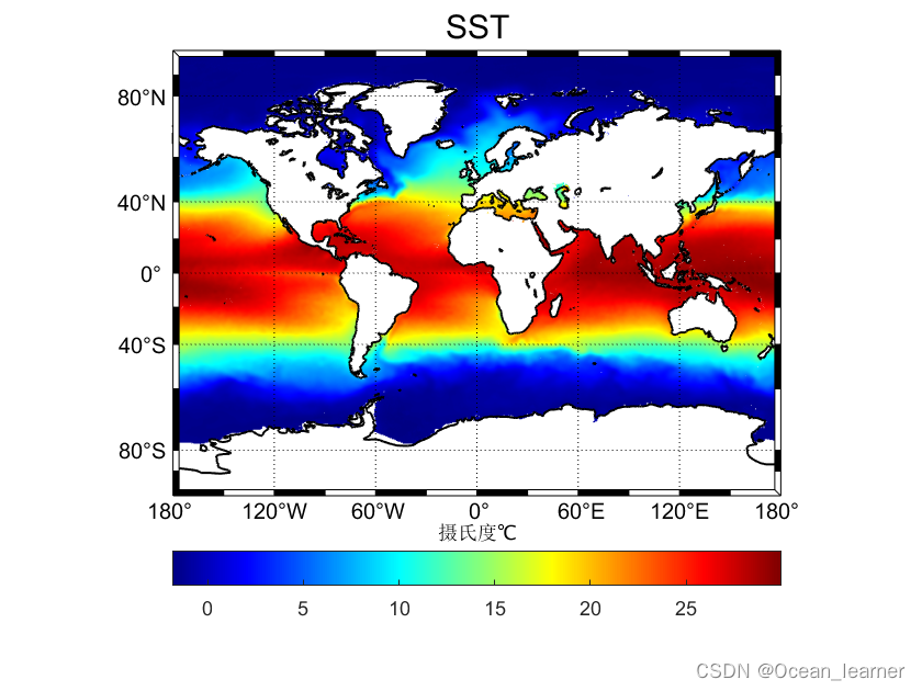 

 over！

本文来自互联网用户投稿，文章观点仅代表作者本人，不代表本站立场，不承担相关法律责任。如若转载，请注明出处。 如若内容造成侵权/违法违规/事实不符，请点击【内容举报】进行投诉反馈！