机器学习/深度学习实战——kaggle房价预测比赛实战(数据分析篇)
文章目录
- 1. 数据分析
- 1.1 训练数据分析
- (1)训练数据前5条数据
- (2)训练数据大小
- (3)训练数据统计信息
- (4)训练数据类型
- (5)训练数据缺失数据统计
- (6)训练数据缺失值可视化
- (7)训练数据缺失值相关性分析
- (8)训练数据标签分布柱状图
- (9)部分属性与房价关系分析(箱状图和散点图)
- 1.2 测试数据分析
- (1) 测试数据前5条数据
- (2) 测试数据类型统计
- (3) 测试数据大小
- (4) 测试数据缺失值统计
- (5) 测试数据缺失值可视化
- (6) 测试数据缺失值相关性分析
- 1.3 训练数据和测试数据对比
- (1) 数据类型对比
- (2) 缺失数据对比
- (3)数据分布统计与对比
- 1) 对比离散数据
- 2)对比连续数据
- 3) 检查数值型特征的线性程度
- 4) 非数值型数据对比分析
- 1.4 数值型数据缺失分析
- 1.5 时序特征分析(包含年月日信息的特征)
- 1.6 数据相关性分析
很不容易,这个实战项目肝了好几天,借鉴了很多大佬的思路和代码,也从中学习到了很多东西(我喜欢将经典的代码复写一遍,感觉这样学习到的东西比CV大法会高一点点),因为这个项目的内容比较多,所以我将会分为4~5个blog进行梳理。
- 第1个blog:数据分析
- 第2个blog:数据预处理
- 第3个blog:应用机器学习回归分析算法进行建模和预测
- 第4个blog:应用pytorch设计深度学习模型
相关:
kaggle 比赛:House Prices - Advanced Regression Techniques
数据下载地址:百度网盘 提取码: w2t6
1. 数据分析
加载原始数据
# 加载原始数据
train_data = pd.read_csv('./data/California house price/house-prices-advanced-regression-techniques/train.csv')
test_data = pd.read_csv('./data/California house price/house-prices-advanced-regression-techniques/test.csv')
combined_df = pd.concat([train_data,test_data],axis=0)
1.1 训练数据分析
(1)训练数据前5条数据
# 查看头5条数据
train_data.head()
| Id | MSSubClass | MSZoning | LotFrontage | LotArea | Street | Alley | LotShape | LandContour | Utilities | ... | PoolArea | PoolQC | Fence | MiscFeature | MiscVal | MoSold | YrSold | SaleType | SaleCondition | SalePrice | |
|---|---|---|---|---|---|---|---|---|---|---|---|---|---|---|---|---|---|---|---|---|---|
| 0 | 1 | 60 | RL | 65.00 | 8450 | Pave | NaN | Reg | Lvl | AllPub | ... | 0 | NaN | NaN | NaN | 0 | 2 | 2008 | WD | Normal | 208500 |
| 1 | 2 | 20 | RL | 80.00 | 9600 | Pave | NaN | Reg | Lvl | AllPub | ... | 0 | NaN | NaN | NaN | 0 | 5 | 2007 | WD | Normal | 181500 |
| 2 | 3 | 60 | RL | 68.00 | 11250 | Pave | NaN | IR1 | Lvl | AllPub | ... | 0 | NaN | NaN | NaN | 0 | 9 | 2008 | WD | Normal | 223500 |
| 3 | 4 | 70 | RL | 60.00 | 9550 | Pave | NaN | IR1 | Lvl | AllPub | ... | 0 | NaN | NaN | NaN | 0 | 2 | 2006 | WD | Abnorml | 140000 |
| 4 | 5 | 60 | RL | 84.00 | 14260 | Pave | NaN | IR1 | Lvl | AllPub | ... | 0 | NaN | NaN | NaN | 0 | 12 | 2008 | WD | Normal | 250000 |
5 rows × 81 columns
(2)训练数据大小
# 训练数据的大小
train_data.shape
(1460, 81)
(3)训练数据统计信息
# 训练数据信息
train_data.info()
RangeIndex: 1460 entries, 0 to 1459
Data columns (total 81 columns):#   Column         Non-Null Count  Dtype
---  ------         --------------  -----  0   Id             1460 non-null   int64  1   MSSubClass     1460 non-null   int64  2   MSZoning       1460 non-null   object 3   LotFrontage    1201 non-null   float644   LotArea        1460 non-null   int64  5   Street         1460 non-null   object 6   Alley          91 non-null     object 7   LotShape       1460 non-null   object 8   LandContour    1460 non-null   object 9   Utilities      1460 non-null   object 10  LotConfig      1460 non-null   object 11  LandSlope      1460 non-null   object 12  Neighborhood   1460 non-null   object 13  Condition1     1460 non-null   object 14  Condition2     1460 non-null   object 15  BldgType       1460 non-null   object 16  HouseStyle     1460 non-null   object 17  OverallQual    1460 non-null   int64  18  OverallCond    1460 non-null   int64  19  YearBuilt      1460 non-null   int64  20  YearRemodAdd   1460 non-null   int64  21  RoofStyle      1460 non-null   object 22  RoofMatl       1460 non-null   object 23  Exterior1st    1460 non-null   object 24  Exterior2nd    1460 non-null   object 25  MasVnrType     1452 non-null   object 26  MasVnrArea     1452 non-null   float6427  ExterQual      1460 non-null   object 28  ExterCond      1460 non-null   object 29  Foundation     1460 non-null   object 30  BsmtQual       1423 non-null   object 31  BsmtCond       1423 non-null   object 32  BsmtExposure   1422 non-null   object 33  BsmtFinType1   1423 non-null   object 34  BsmtFinSF1     1460 non-null   int64  35  BsmtFinType2   1422 non-null   object 36  BsmtFinSF2     1460 non-null   int64  37  BsmtUnfSF      1460 non-null   int64  38  TotalBsmtSF    1460 non-null   int64  39  Heating        1460 non-null   object 40  HeatingQC      1460 non-null   object 41  CentralAir     1460 non-null   object 42  Electrical     1459 non-null   object 43  1stFlrSF       1460 non-null   int64  44  2ndFlrSF       1460 non-null   int64  45  LowQualFinSF   1460 non-null   int64  46  GrLivArea      1460 non-null   int64  47  BsmtFullBath   1460 non-null   int64  48  BsmtHalfBath   1460 non-null   int64  49  FullBath       1460 non-null   int64  50  HalfBath       1460 non-null   int64  51  BedroomAbvGr   1460 non-null   int64  52  KitchenAbvGr   1460 non-null   int64  53  KitchenQual    1460 non-null   object 54  TotRmsAbvGrd   1460 non-null   int64  55  Functional     1460 non-null   object 56  Fireplaces     1460 non-null   int64  57  FireplaceQu    770 non-null    object 58  GarageType     1379 non-null   object 59  GarageYrBlt    1379 non-null   float6460  GarageFinish   1379 non-null   object 61  GarageCars     1460 non-null   int64  62  GarageArea     1460 non-null   int64  63  GarageQual     1379 non-null   object 64  GarageCond     1379 non-null   object 65  PavedDrive     1460 non-null   object 66  WoodDeckSF     1460 non-null   int64  67  OpenPorchSF    1460 non-null   int64  68  EnclosedPorch  1460 non-null   int64  69  3SsnPorch      1460 non-null   int64  70  ScreenPorch    1460 non-null   int64  71  PoolArea       1460 non-null   int64  72  PoolQC         7 non-null      object 73  Fence          281 non-null    object 74  MiscFeature    54 non-null     object 75  MiscVal        1460 non-null   int64  76  MoSold         1460 non-null   int64  77  YrSold         1460 non-null   int64  78  SaleType       1460 non-null   object 79  SaleCondition  1460 non-null   object 80  SalePrice      1460 non-null   int64
dtypes: float64(3), int64(35), object(43)
memory usage: 924.0+ KB
(4)训练数据类型
# 训练数据类型统计
train_dtype = train_data.dtypes
train_dtype.value_counts()
object 43int64 35float64 3dtype: int64
(5)训练数据缺失数据统计
# 训练数据中的空值排序前20个
train_data.isnull().sum().sort_values(ascending=False).head(20)
PoolQC 1453MiscFeature 1406Alley 1369Fence 1179FireplaceQu 690LotFrontage 259GarageCond 81GarageType 81GarageYrBlt 81GarageFinish 81GarageQual 81BsmtExposure 38BsmtFinType2 38BsmtFinType1 37BsmtCond 37BsmtQual 37MasVnrArea 8MasVnrType 8Electrical 1Utilities 0dtype: int64
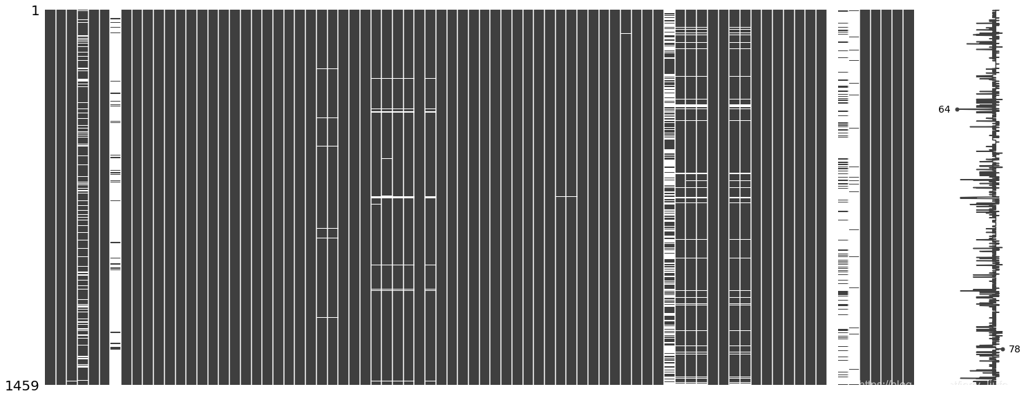
(6)训练数据缺失值可视化
# 使用Misingno可视化缺失数据
msno.matrix(train_data)

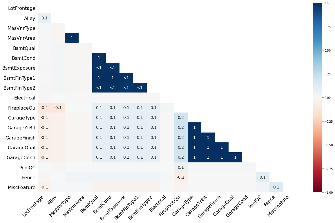
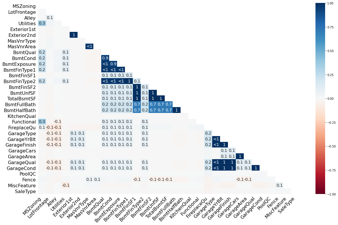
(7)训练数据缺失值相关性分析
# 使用misingno查看缺失数据之间的相关性:表征一个变量的存在和不存在如何强烈地影响另一个的存在
# (比如说如果rate1和rate2的热度值是1,那么rate11缺失,rate2也必然缺失,两者在缺失性之间是直接相关的)
msno.heatmap(train_data)
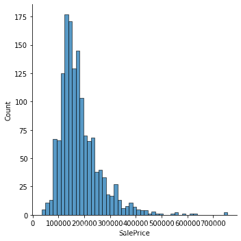
(8)训练数据标签分布柱状图
# 查看训练数据对应价格的分布
sns.displot(train_data['SalePrice'])
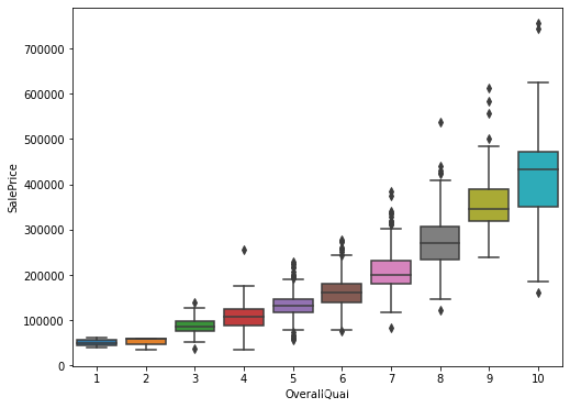
(9)部分属性与房价关系分析(箱状图和散点图)
查看对房屋的整体评价和价格之箱状图:箱状图不受异常值的影响,可以相对稳定地描述数据的离散分布情况

# 可以看到整体评分越高其价格是越高的
overallQual_SalePrice = pd.concat([train_data['SalePrice'],train_data['OverallQual']],axis=1)
plt.figure(figsize=(8,6))
sns.boxplot(x='OverallQual',y='SalePrice',data=overallQual_SalePrice)
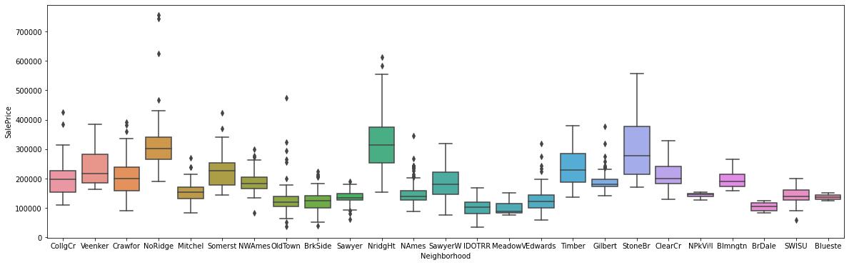
# 用箱状图查看一下离散非数值型数据的分布
# 可以看到如果neighorhood是在stoneBr和NridgHt附近的话,价格会较高
Neighborhood_SalePrice = pd.concat([train_data['SalePrice'],train_data['Neighborhood']],axis=1)
plt.figure(figsize=(20,6))
sns.boxplot(x='Neighborhood',y='SalePrice',data=Neighborhood_SalePrice)
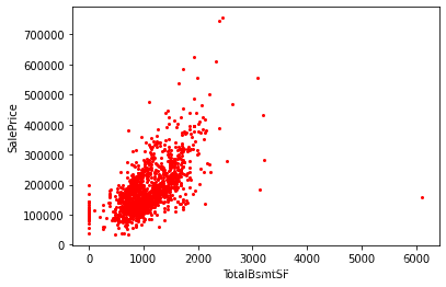
# 绘制和价格相关的特征的散点图
TotalBsmtSF_SalePrice = pd.concat([train_data['SalePrice'],train_data['TotalBsmtSF']],axis=1)
plt.figure(figsize=(8,6))
TotalBsmtSF_SalePrice.plot.scatter(x='TotalBsmtSF',y='SalePrice',s=4,c='red')
1.2 测试数据分析
(1) 测试数据前5条数据
test_data.head()
| Id | MSSubClass | MSZoning | LotFrontage | LotArea | Street | Alley | LotShape | LandContour | Utilities | ... | ScreenPorch | PoolArea | PoolQC | Fence | MiscFeature | MiscVal | MoSold | YrSold | SaleType | SaleCondition | |
|---|---|---|---|---|---|---|---|---|---|---|---|---|---|---|---|---|---|---|---|---|---|
| 0 | 1461 | 20 | RH | 80.00 | 11622 | Pave | NaN | Reg | Lvl | AllPub | ... | 120 | 0 | NaN | MnPrv | NaN | 0 | 6 | 2010 | WD | Normal |
| 1 | 1462 | 20 | RL | 81.00 | 14267 | Pave | NaN | IR1 | Lvl | AllPub | ... | 0 | 0 | NaN | NaN | Gar2 | 12500 | 6 | 2010 | WD | Normal |
| 2 | 1463 | 60 | RL | 74.00 | 13830 | Pave | NaN | IR1 | Lvl | AllPub | ... | 0 | 0 | NaN | MnPrv | NaN | 0 | 3 | 2010 | WD | Normal |
| 3 | 1464 | 60 | RL | 78.00 | 9978 | Pave | NaN | IR1 | Lvl | AllPub | ... | 0 | 0 | NaN | NaN | NaN | 0 | 6 | 2010 | WD | Normal |
| 4 | 1465 | 120 | RL | 43.00 | 5005 | Pave | NaN | IR1 | HLS | AllPub | ... | 144 | 0 | NaN | NaN | NaN | 0 | 1 | 2010 | WD | Normal |
5 rows × 80 columns
(2) 测试数据类型统计
# 查看测试数据中的数据类型统计
test_dtype = test_data.dtypes
test_dtype.value_counts()
object     43
int64      26
float64    11
dtype: int64
(3) 测试数据大小
test_data.shape
(1459, 80)
(4) 测试数据缺失值统计
test_data.isnull().sum().sort_values(ascending = False).head(20)
PoolQC          1456
MiscFeature     1408
Alley           1352
Fence           1169
FireplaceQu      730
LotFrontage      227
GarageCond        78
GarageQual        78
GarageYrBlt       78
GarageFinish      78
GarageType        76
BsmtCond          45
BsmtQual          44
BsmtExposure      44
BsmtFinType1      42
BsmtFinType2      42
MasVnrType        16
MasVnrArea        15
MSZoning           4
BsmtHalfBath       2
dtype: int64
(5) 测试数据缺失值可视化
msno.matrix(test_data)
(6) 测试数据缺失值相关性分析
# 从这里看出:其实我们的测试数据缺失比训练数据更加严重
msno.heatmap(test_data)
1.3 训练数据和测试数据对比
(1) 数据类型对比
主要发现一些数据类型是int64和float64的区别,对于我们的影响不是很大
# 将标签值SalePrice去除,然后使用pandas的compare将两个dataframe进行比较
train_dtype = train_dtype.drop('SalePrice')
train_dtype.compare(test_dtype)
| self | other | |
|---|---|---|
| BsmtFinSF1 | int64 | float64 |
| BsmtFinSF2 | int64 | float64 |
| BsmtUnfSF | int64 | float64 |
| TotalBsmtSF | int64 | float64 |
| BsmtFullBath | int64 | float64 |
| BsmtHalfBath | int64 | float64 |
| GarageCars | int64 | float64 |
| GarageArea | int64 | float64 |
(2) 缺失数据对比
null_train = train_data.isnull().sum()
null_test = test_data.isnull().sum()
null_train = null_train.drop('SalePrice')
null_comp_df = null_train.compare(null_test).sort_values(['self'],ascending=[False])
null_comp_df
| self | other | |
|---|---|---|
| PoolQC | 1453.00 | 1456.00 |
| MiscFeature | 1406.00 | 1408.00 |
| Alley | 1369.00 | 1352.00 |
| Fence | 1179.00 | 1169.00 |
| FireplaceQu | 690.00 | 730.00 |
| LotFrontage | 259.00 | 227.00 |
| GarageType | 81.00 | 76.00 |
| GarageCond | 81.00 | 78.00 |
| GarageYrBlt | 81.00 | 78.00 |
| GarageFinish | 81.00 | 78.00 |
| GarageQual | 81.00 | 78.00 |
| BsmtFinType2 | 38.00 | 42.00 |
| BsmtExposure | 38.00 | 44.00 |
| BsmtFinType1 | 37.00 | 42.00 |
| BsmtCond | 37.00 | 45.00 |
| BsmtQual | 37.00 | 44.00 |
| MasVnrArea | 8.00 | 15.00 |
| MasVnrType | 8.00 | 16.00 |
| Electrical | 1.00 | 0.00 |
| GarageArea | 0.00 | 1.00 |
| GarageCars | 0.00 | 1.00 |
| MSZoning | 0.00 | 4.00 |
| Functional | 0.00 | 2.00 |
| KitchenQual | 0.00 | 1.00 |
| BsmtHalfBath | 0.00 | 2.00 |
| BsmtFullBath | 0.00 | 2.00 |
| TotalBsmtSF | 0.00 | 1.00 |
| BsmtUnfSF | 0.00 | 1.00 |
| BsmtFinSF2 | 0.00 | 1.00 |
| BsmtFinSF1 | 0.00 | 1.00 |
| Exterior2nd | 0.00 | 1.00 |
| Exterior1st | 0.00 | 1.00 |
| Utilities | 0.00 | 2.00 |
| SaleType | 0.00 | 1.00 |
(3)数据分布统计与对比
统计数据类别数量:
-
1)数值型特征数量
- 离散特征数量(如果非独立数值少于25个认为该特征为离散特征)
- 连续特征数量
-
2)非数值型数据数量
numerical_features = [col for col in train_data.columns if train_data[col].dtypes != 'O']
discrete_features = [col for col in numerical_features if len(train_data[col].unique()) < 25 and col not in ['Id']]
continuous_features = [feature for feature in numerical_features if feature not in discrete_features+['Id']]
categorical_features = [col for col in train_data.columns if train_data[col].dtype == 'O']print("Total Number of Numerical Columns : ",len(numerical_features))
print("Number of discrete features : ",len(discrete_features))
print("No of continuous features are : ", len(continuous_features))
print("Number of non-numeric features : ",len(categorical_features))
Total Number of Numerical Columns :  38
Number of discrete features :  18
No of continuous features are :  19
Number of non-numeric features :  43
插入一个名为Label标识训练数据和测试数据的特征
combined_df['Label'] = "test"
combined_df['Label'][:1460] = "Train"
1) 对比离散数据
# 对比离散数据
"""
sns.hitplot(data,x,y,hue,ax)
data:pandas.Dataframe,numpy.ndarray,mapping,or sequence:input data
x,y : 指定x,y轴的变量
hue:确定绘图颜色的变量
ax:预先定义的绘图区域
"""
f,axes = plt.subplots(3,6,figsize=(30,10),sharex=False)
for i,feature in enumerate(discrete_features):sns.histplot(data=combined_df,x=feature,hue='Label',ax=axes[i%3,i//3])
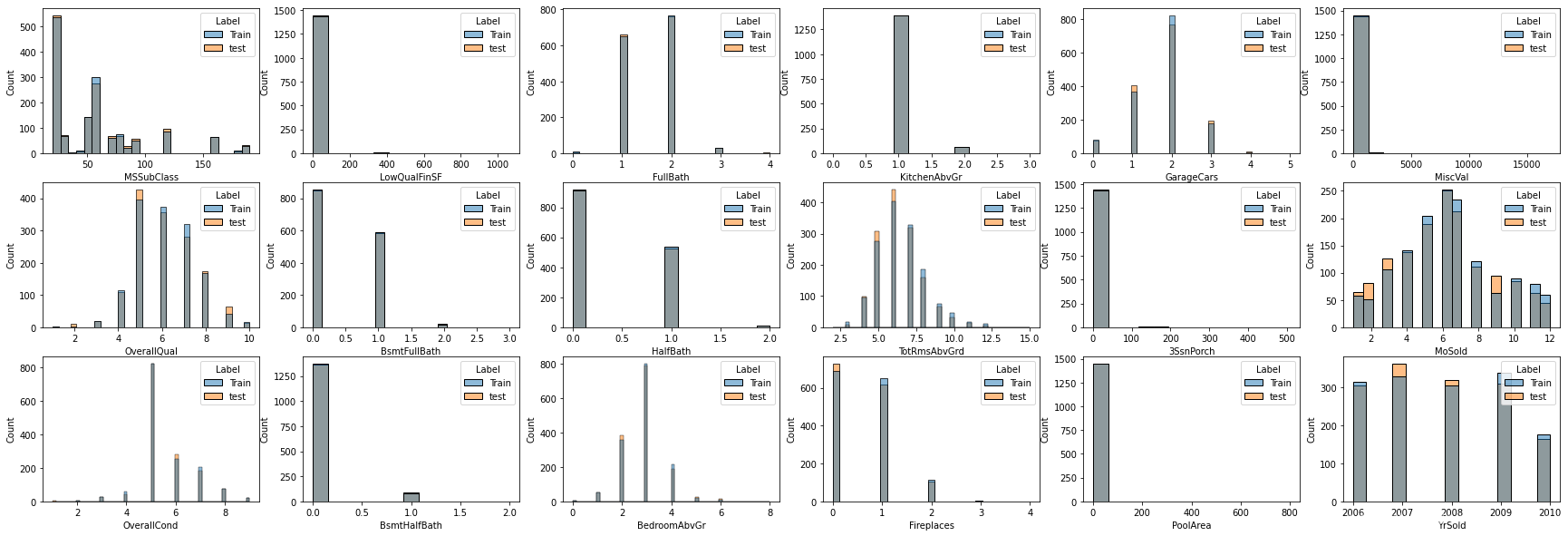
上面离散分布的数据说明:
- 很多数据可以重新分类为分类数据(非数值型数据),例如
MSSublass - 很多特征以0和null值为主(例如
PoolArea,LowQualFinSF,3SsnPorch,MiscVal),因此也以考虑将这些特征删除
2)对比连续数据
#对比连续数据
f,axes = plt.subplots(4,6,figsize=(30,15),sharex=False)
for i,feature in enumerate(continuous_features):sns.histplot(data=combined_df,x=feature,hue='Label',ax=axes[i%4,i//4])

上述连续数据对比说明:
- 对于连续数据:训练和测试数据的分布都基本相同
3) 检查数值型特征的线性程度
# 检查数值数据的线性分布
"""
横轴为数值数据特征,纵轴为价格标签
"""
f,axes = plt.subplots(7,6,figsize=(30,30),sharex=False)
for i,feature in enumerate(numerical_features):sns.scatterplot(data=combined_df,x=feature,y="SalePrice",ax=axes[i%7,i//7])
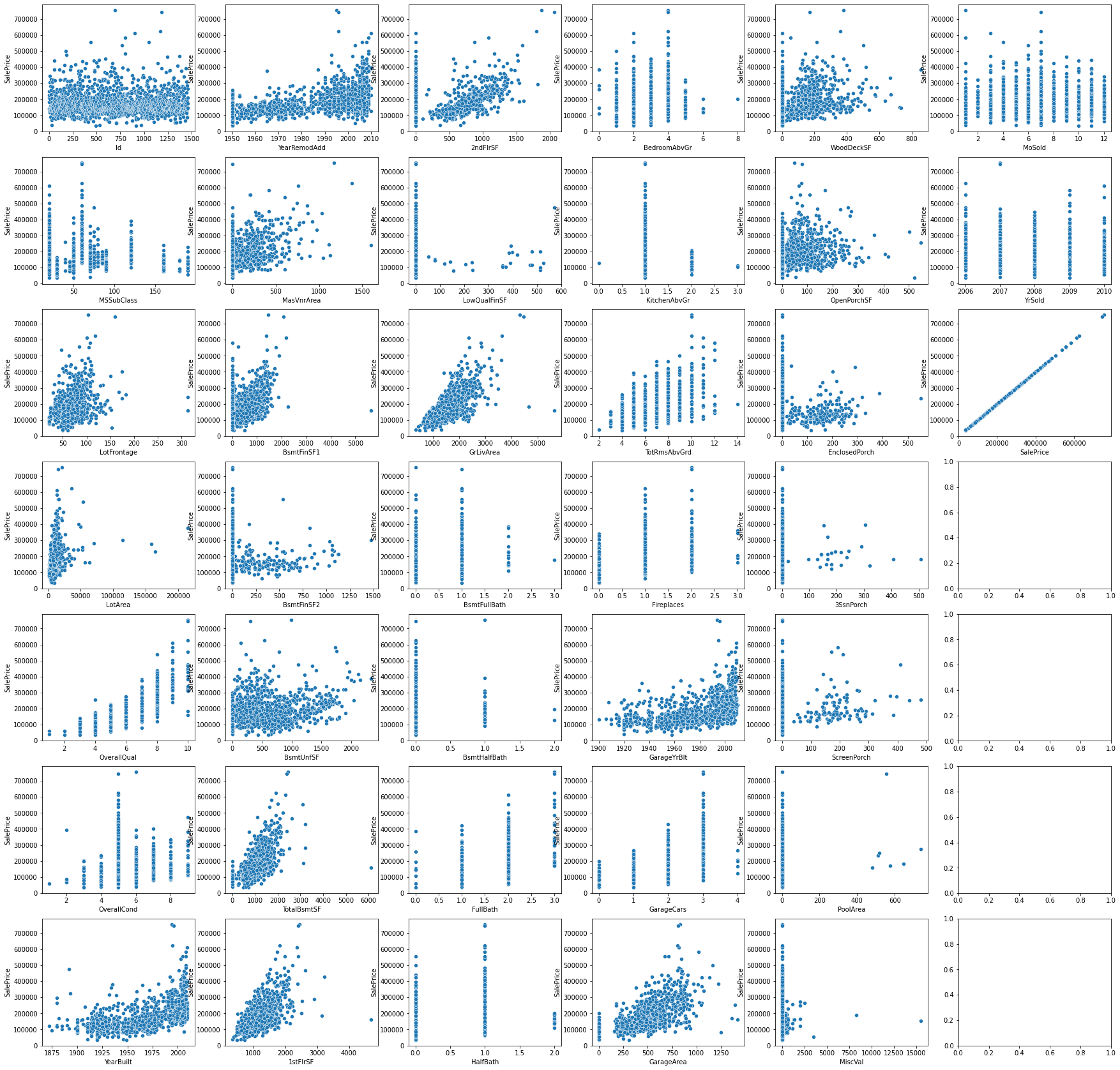
从上面可以发现很多特征关于价格标签并非是线性的:
- ‘SalePrice’ VS.‘BsmtUnfSF’,
- ‘SalePrice’ VS.‘TotalBsmtSF’,
- ‘SalePrice’ VS.‘GarageArea’,
- ‘SalePrice’ VS.‘LotArea’,
- ‘SalePrice’ VS.‘LotFrontage’,
- ‘SalePrice’ VS.‘GrLivArea’,
- ‘SalePrice’ VS.‘1stFlrSF’,
4) 非数值型数据对比分析
# 对比非数值型数据对比分析
f,axes = plt.subplots(7,7,figsize=(30,30),sharex=False)
for i,feature in enumerate(categorical_features):sns.countplot(data=combined_df,x=feature,hue="Label",ax=axes[i%7,i//7])
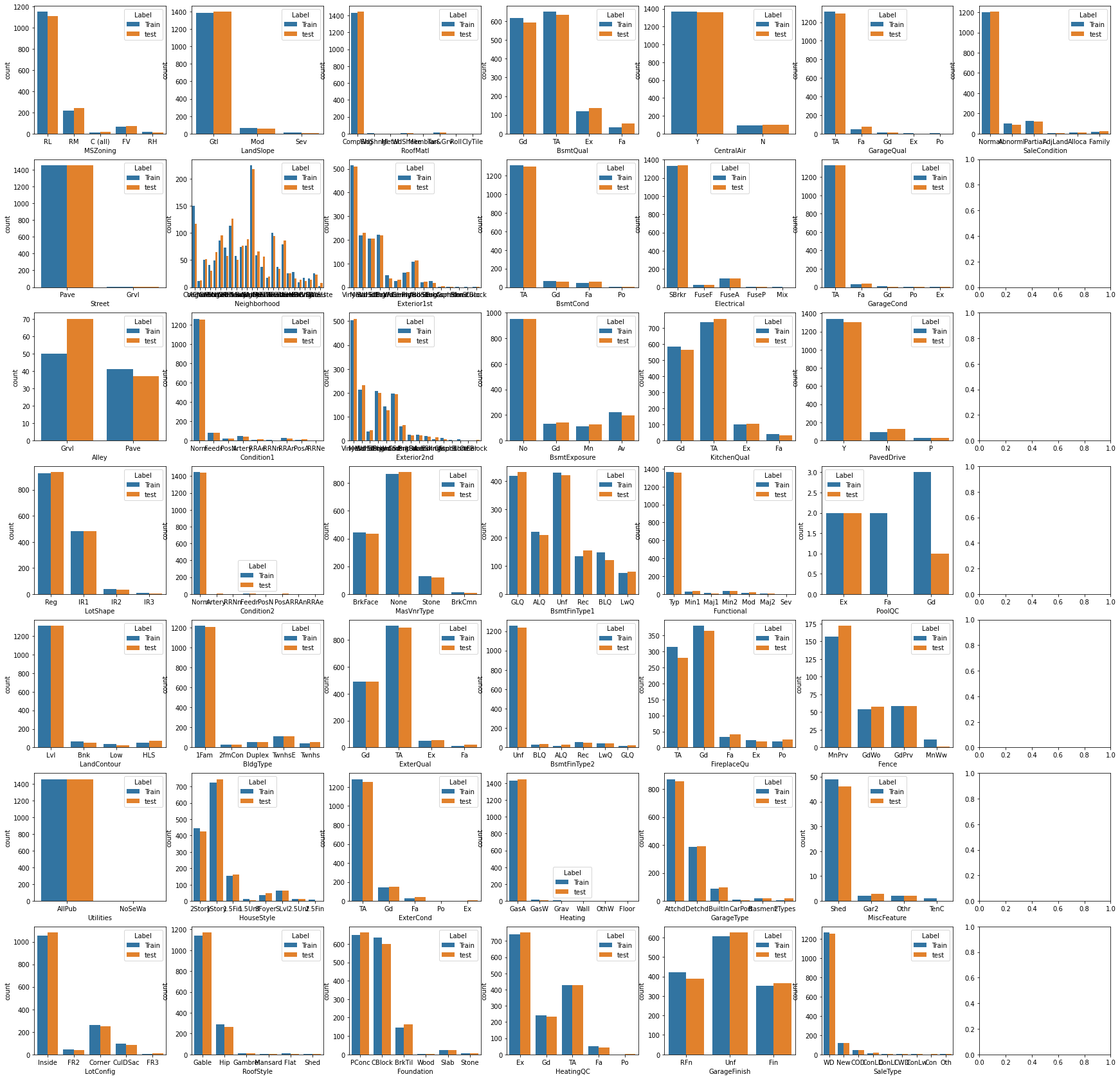
统计非数值型数据的对比统计结果:
- 对于大多数特征而言,训练和测试数据的分布是类似的
- 一些特征存在主要的项目,可以考虑将一些次要项目合并在一起或者将这些列给删掉
- ‘RoofMatl’,‘Street’,‘Condition2’,‘Utilities’,‘Heating’ (这些列应该删掉)
- ‘Fa’ & ‘Po’ 在 ‘HeatingQC’, ‘FireplaceQu’, ‘GarageQual’ and 'GarageCond’这些特征中或许可以考虑将其合并
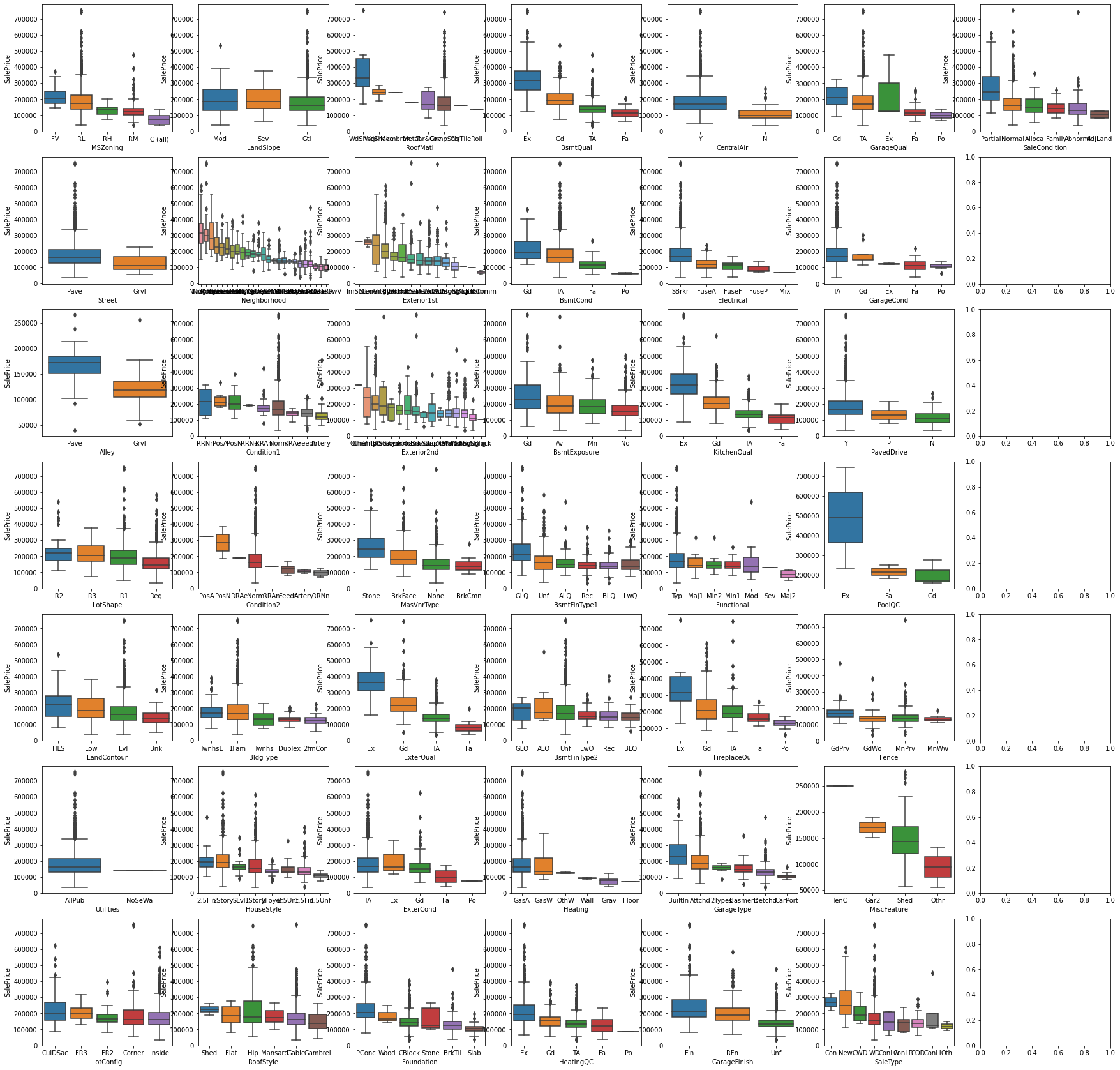
# 通过箱状图分析非数值型数据的分布(值取的对应价格)
f, axes = plt.subplots(7,7 , figsize=(30, 30), sharex=False)
for i, feature in enumerate(categorical_features):sort_list = sorted(combined_df.groupby(feature)['SalePrice'].median().items(), key= lambda x:x[1], reverse = True)order_list = [x[0] for x in sort_list ]sns.boxplot(data = combined_df, x = feature, y = 'SalePrice', order=order_list, ax=axes[i%7, i//7])
plt.show()
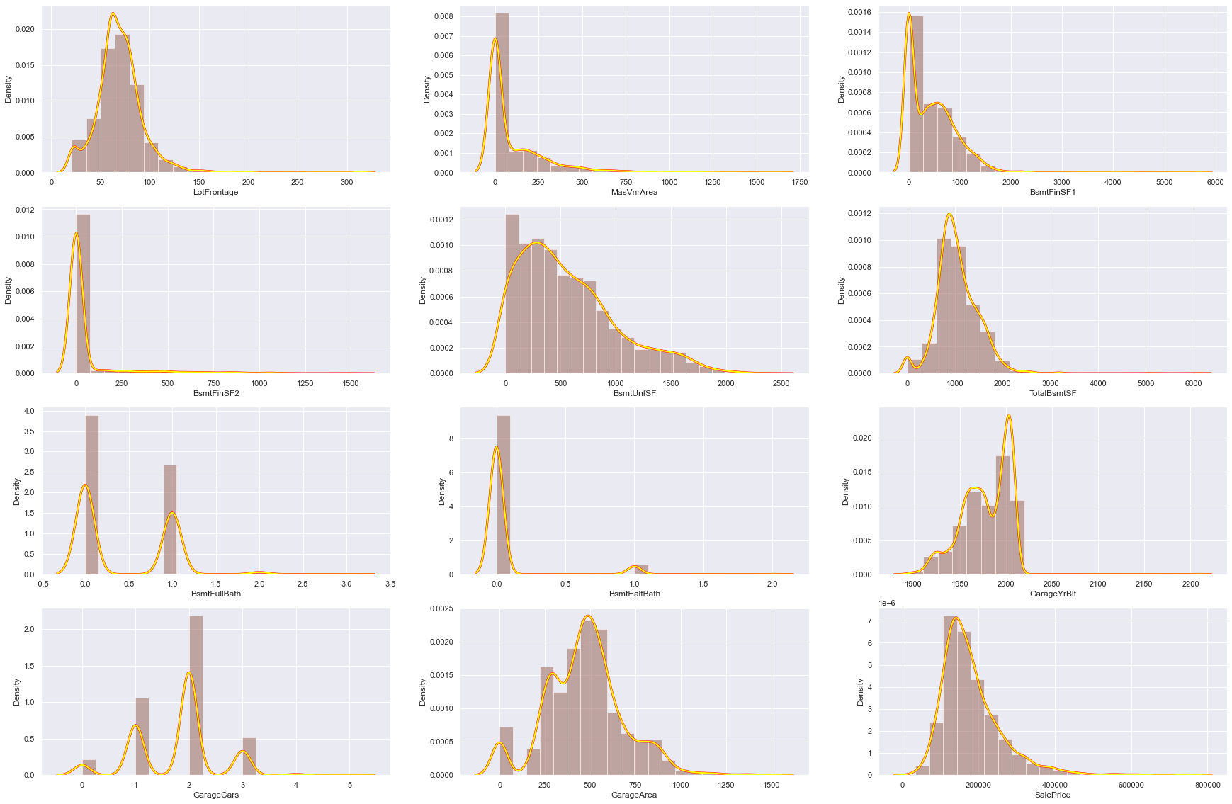
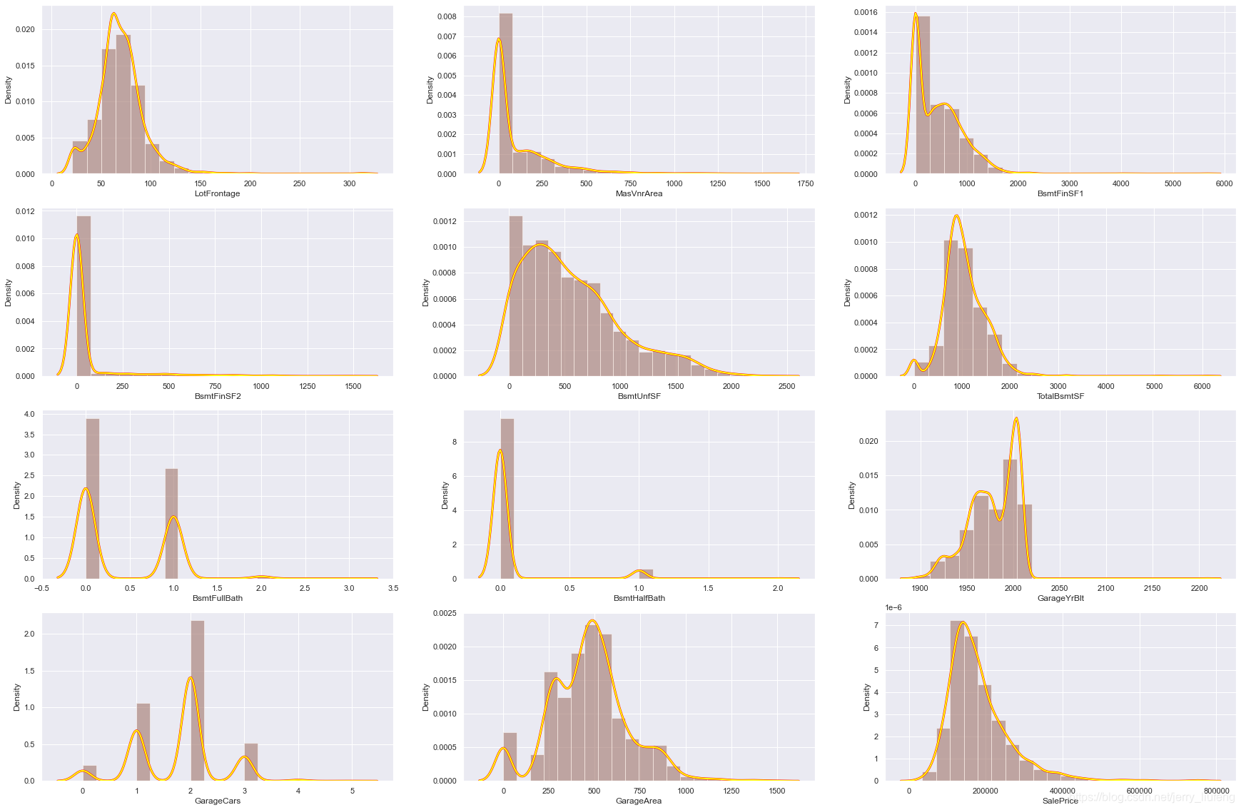
1.4 数值型数据缺失分析
# 检查数值型数据的分布特征并填充均值
null_features_numerical = [col for col in combined_df.columns if combined_df[col].isnull().sum()>0 and col not in categorical_features]
plt.figure(figsize=(30,20))
sns.set()warnings.simplefilter('ignore')
for i,var in enumerate(null_features_numerical):plt.subplot(4,3,i+1)sns.distplot(combined_df[var],bins=20,kde_kws={'linewidth':3,'color':'red'},label="original")sns.distplot(combined_df[var],bins=20,kde_kws={'linewidth':2,'color':'yellow'},label="mean")
# # 检查数值型数据的分布特征并填充中位值
plt.figure(figsize=(30,20))
sns.set()
warnings.simplefilter("ignore")
for i,var in enumerate(null_features_numerical):plt.subplot(4,3,i+1)sns.distplot(combined_df[var],bins=20,kde_kws={'linewidth':3,'color':'red'},label="original")sns.distplot(combined_df[var],bins=20,kde_kws={'linewidth':2,'color':'yellow'},label="median")
1.5 时序特征分析(包含年月日信息的特征)
year_feature = [col for col in combined_df.columns if "Yr" in col or 'Year' in col]
year_feature
['YearBuilt', 'YearRemodAdd', 'GarageYrBlt', 'YrSold']
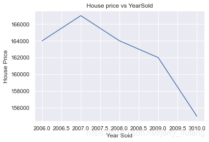
# 然后检查一下这些特征与销售价格是否有关系
combined_df.groupby('YrSold')['SalePrice'].median().plot() # groupby().median()表示取每一组的中位数
plt.xlabel('Year Sold')
plt.ylabel('House Price')
plt.title('House price vs YearSold')
Text(0.5, 1.0, 'House price vs YearSold')
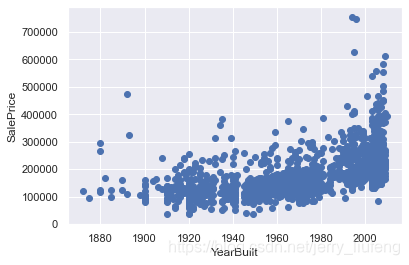
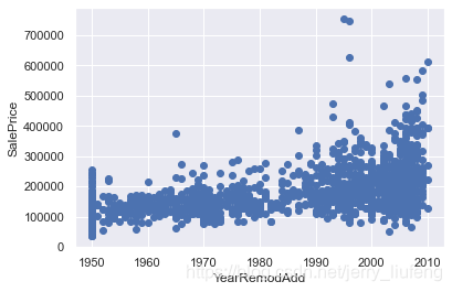
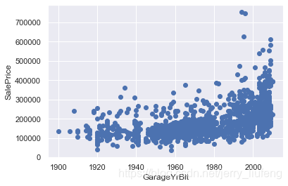
# 绘制其他三个特征与销售价格的散点对应图
# 可以看到随着时间的增加,价格是逐增加的
for feature in year_feature:if feature != 'YrSold':hs = combined_df.copy()plt.scatter(hs[feature],hs['SalePrice'])plt.xlabel(feature)plt.ylabel('SalePrice')plt.show()
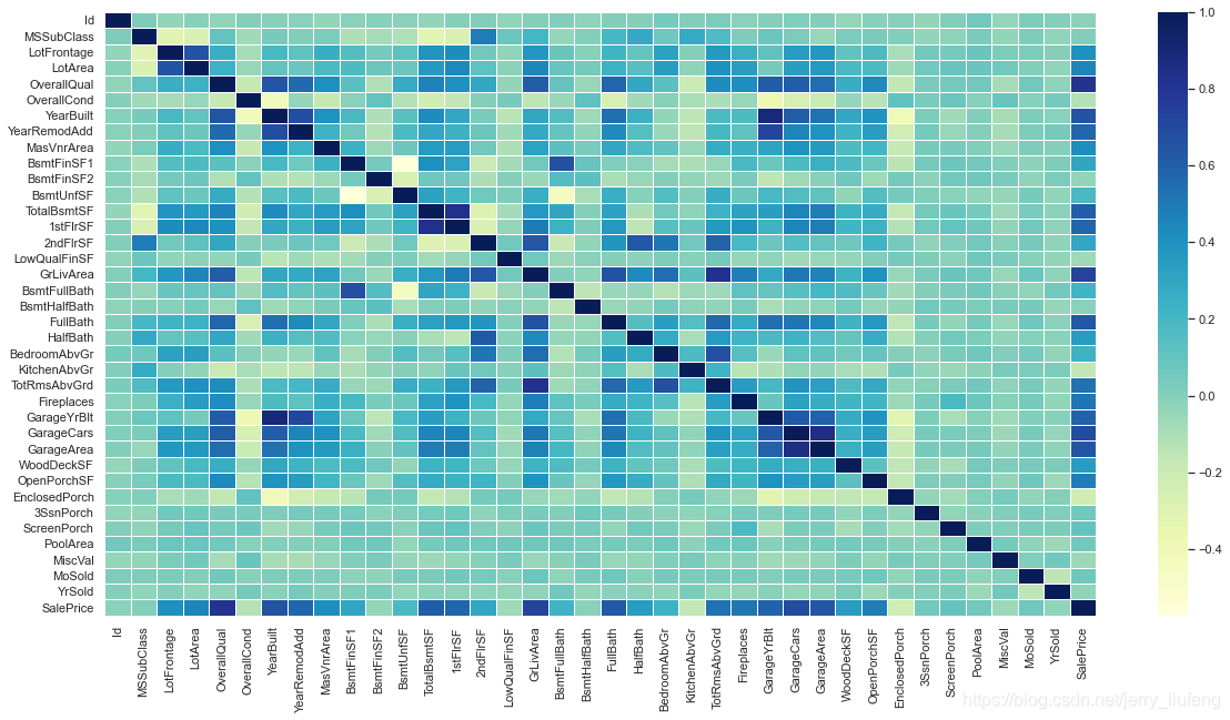
1.6 数据相关性分析
# 使用热力图查看特征之间的相互关系
corrmat = train_data.corr(method='spearman') # 计算不同数据之间的相系数
plt.figure(figsize=(20,10))
sns.heatmap(corrmat,cmap="YlGnBu", linewidths=.5)
本文来自互联网用户投稿,文章观点仅代表作者本人,不代表本站立场,不承担相关法律责任。如若转载,请注明出处。 如若内容造成侵权/违法违规/事实不符,请点击【内容举报】进行投诉反馈!