目录

第一部分 代码实现

1.1数据准备，并引入基本函数库

1.2 定义 HybridSN 类

1.3 创建数据集

1.4 开始训练

1.5 模型测试和备用函数

第二部分 问题思考

第一部分 代码实现

  本次代码实现了混合网络解决高光谱图像分类问题，均在Colab中完成。

1.1数据准备，并引入基本函数库

准备之前，由于一直下载不了数据，这里对python版本进了一个改动并且把wget的版本进行了一个更新

!apt-get install python3.6
!wget https://ftp.gnu.org/gnu/wget/wget-1.21.1.tar.gz
!tar -xzf wget-1.21.1.tar.gz
!sudo apt-get install libgnutls28-dev
!cd wget-1.21.1 && ./configure && make && make install

取得Indian_pines相关数据

! wget http://www.ehu.eus/ccwintco/uploads/6/67/Indian_pines_corrected.mat
! wget http://www.ehu.eus/ccwintco/uploads/c/c4/Indian_pines_gt.mat
! pip install spectral

引入基本函数库

##引入基本函数库import numpy as np
import matplotlib.pyplot as plt
import scipy.io as sio
from sklearn.decomposition import PCA
from sklearn.model_selection import train_test_split
from sklearn.metrics import confusion_matrix, accuracy_score, classification_report, cohen_kappa_score
import spectral
import torch
import torchvision
import torch.nn as nn
import torch.nn.functional as F
import torch.optim as optim

1.2 定义 HybridSN 类

  根据《HybridSN: Exploring 3-D–2-DCNN Feature Hierarchy for Hyperspectral Image Classification》论文内容，定义相关HybridSN类

##定义 HybridSN 类class_num = 16class HybridSN(nn.Module):def __init__(self, num_classes=16):super(HybridSN, self).__init__()# conv1：（1, 30, 25, 25）， 8个 7x3x3 的卷积核 ==>（8, 24, 23, 23）self.conv1 = nn.Conv3d(1, 8, (7, 3, 3))# conv2：（8, 24, 23, 23）， 16个 5x3x3 的卷积核 ==>（16, 20, 21, 21）self.conv2 = nn.Conv3d(8, 16, (5, 3, 3))# conv3：（16, 20, 21, 21），32个 3x3x3 的卷积核 ==>（32, 18, 19, 19）self.conv3 = nn.Conv3d(16, 32, (3, 3, 3))# conv3_2d （576, 19, 19），64个 3x3 的卷积核 ==>（（64, 17, 17）self.conv3_2d = nn.Conv2d(576, 64, (3,3))# 全连接层（256个节点）self.dense1 =  nn.Linear(18496,256)# 全连接层（128个节点）self.dense2 =  nn.Linear(256,128)# 最终输出层(16个节点)self.out = nn.Linear(128, num_classes)#  Dropout（0.4)self.drop = nn.Dropout(p=0.4)#######################这里是优化的方向（一会还会添加注意力机制）#######################软最大化self.soft = nn.LogSoftmax(dim=1)#self.soft = nn.Softmax(dim=1)#加入BN归一化数据self.bn1=nn.BatchNorm3d(8)self.bn2=nn.BatchNorm3d(16)self.bn3=nn.BatchNorm3d(32)self.bn4=nn.BatchNorm2d(64)# 激活函数ReLUself.relu = nn.ReLU()###########################################定义完了各个模块，记得在这里调用执行：def forward(self, x):out = self.relu(self.conv1(x))#out = self.bn1(out)#BN层out = self.relu(self.conv2(out))#out = self.bn2(out)#BN层out = self.relu(self.conv3(out))#out = self.bn3(out)#BN层out = out.view(-1, out.shape[1] * out.shape[2], out.shape[3], out.shape[4])# 进行二维卷积，因此把前面的 32*18 reshape 一下，得到 （576, 19, 19）#out = self.attention(out)#调用注意力机制out = self.relu(self.conv3_2d(out))#out = self.bn4(out)#BN层# flatten 操作，变为 18496 维的向量，out = out.view(out.size(0), -1)out = self.dense1(out)out = self.drop(out)out = self.dense2(out)out = self.drop(out)out = self.out(out)out = self.soft(out)return out

1.3 创建数据集

首先对高光谱数据实施PCA降维；然后创建 keras 方便处理的数据格式；然后随机抽取 10% 数据做为训练集，剩余的做为测试集。

首先定义基本函数：

# 对高光谱数据 X 应用 PCA 变换
def applyPCA(X, numComponents):newX = np.reshape(X, (-1, X.shape[2]))pca = PCA(n_components=numComponents, whiten=True)newX = pca.fit_transform(newX)newX = np.reshape(newX, (X.shape[0], X.shape[1], numComponents))return newX# 对单个像素周围提取 patch 时，边缘像素就无法取了，因此，给这部分像素进行 padding 操作
def padWithZeros(X, margin=2):newX = np.zeros((X.shape[0] + 2 * margin, X.shape[1] + 2* margin, X.shape[2]))x_offset = marginy_offset = marginnewX[x_offset:X.shape[0] + x_offset, y_offset:X.shape[1] + y_offset, :] = Xreturn newX# 在每个像素周围提取 patch ，然后创建成符合 keras 处理的格式
def createImageCubes(X, y, windowSize=5, removeZeroLabels = True):# 给 X 做 paddingmargin = int((windowSize - 1) / 2)zeroPaddedX = padWithZeros(X, margin=margin)# split patchespatchesData = np.zeros((X.shape[0] * X.shape[1], windowSize, windowSize, X.shape[2]))patchesLabels = np.zeros((X.shape[0] * X.shape[1]))patchIndex = 0for r in range(margin, zeroPaddedX.shape[0] - margin):for c in range(margin, zeroPaddedX.shape[1] - margin):patch = zeroPaddedX[r - margin:r + margin + 1, c - margin:c + margin + 1]   patchesData[patchIndex, :, :, :] = patchpatchesLabels[patchIndex] = y[r-margin, c-margin]patchIndex = patchIndex + 1if removeZeroLabels:patchesData = patchesData[patchesLabels>0,:,:,:]patchesLabels = patchesLabels[patchesLabels>0]patchesLabels -= 1return patchesData, patchesLabelsdef splitTrainTestSet(X, y, testRatio, randomState=345):X_train, X_test, y_train, y_test = train_test_split(X, y, test_size=testRatio, random_state=randomState, stratify=y)return X_train, X_test, y_train, y_test

下面读取并创建数据集：

# 地物类别
class_num = 16
X = sio.loadmat('Indian_pines_corrected.mat')['indian_pines_corrected']
y = sio.loadmat('Indian_pines_gt.mat')['indian_pines_gt']# 用于测试样本的比例
test_ratio = 0.90
# 每个像素周围提取 patch 的尺寸
patch_size = 25
# 使用 PCA 降维，得到主成分的数量
pca_components = 30print('Hyperspectral data shape: ', X.shape)
print('Label shape: ', y.shape)print('\n... ... PCA tranformation ... ...')
X_pca = applyPCA(X, numComponents=pca_components)
print('Data shape after PCA: ', X_pca.shape)print('\n... ... create data cubes ... ...')
X_pca, y = createImageCubes(X_pca, y, windowSize=patch_size)
print('Data cube X shape: ', X_pca.shape)
print('Data cube y shape: ', y.shape)print('\n... ... create train & test data ... ...')
Xtrain, Xtest, ytrain, ytest = splitTrainTestSet(X_pca, y, test_ratio)
print('Xtrain shape: ', Xtrain.shape)
print('Xtest  shape: ', Xtest.shape)# 改变 Xtrain, Ytrain 的形状，以符合 keras 的要求
Xtrain = Xtrain.reshape(-1, patch_size, patch_size, pca_components, 1)
Xtest  = Xtest.reshape(-1, patch_size, patch_size, pca_components, 1)
print('before transpose: Xtrain shape: ', Xtrain.shape) 
print('before transpose: Xtest  shape: ', Xtest.shape) # 为了适应 pytorch 结构，数据要做 transpose
Xtrain = Xtrain.transpose(0, 4, 3, 1, 2)
Xtest  = Xtest.transpose(0, 4, 3, 1, 2)
print('after transpose: Xtrain shape: ', Xtrain.shape) 
print('after transpose: Xtest  shape: ', Xtest.shape) """ Training dataset"""
class TrainDS(torch.utils.data.Dataset): def __init__(self):self.len = Xtrain.shape[0]self.x_data = torch.FloatTensor(Xtrain)self.y_data = torch.LongTensor(ytrain)        def __getitem__(self, index):# 根据索引返回数据和对应的标签return self.x_data[index], self.y_data[index]def __len__(self): # 返回文件数据的数目return self.len""" Testing dataset"""
class TestDS(torch.utils.data.Dataset): def __init__(self):self.len = Xtest.shape[0]self.x_data = torch.FloatTensor(Xtest)self.y_data = torch.LongTensor(ytest)def __getitem__(self, index):# 根据索引返回数据和对应的标签return self.x_data[index], self.y_data[index]def __len__(self): # 返回文件数据的数目return self.len# 创建 trainloader 和 testloader
trainset = TrainDS()
testset  = TestDS()
train_loader = torch.utils.data.DataLoader(dataset=trainset, batch_size=128, shuffle=True, num_workers=2)
test_loader  = torch.utils.data.DataLoader(dataset=testset,  batch_size=128, shuffle=False, num_workers=2)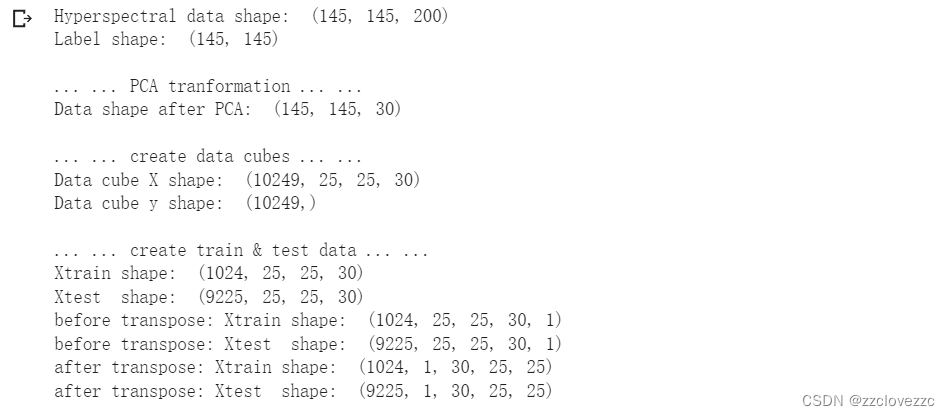

1.4 开始训练

# 使用GPU训练，可以在菜单 "代码执行工具" -> "更改运行时类型" 里进行设置
device = torch.device("cuda:0" if torch.cuda.is_available() else "cpu")# 网络放到GPU上
net = HybridSN().to(device)
criterion = nn.CrossEntropyLoss()
optimizer = optim.Adam(net.parameters(), lr=0.001)# 开始训练
total_loss = 0
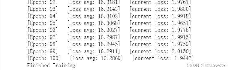
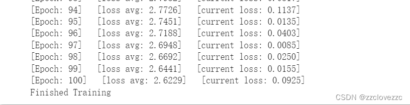
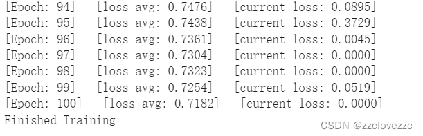
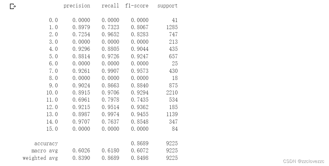
for epoch in range(100):for i, (inputs, labels) in enumerate(train_loader):inputs = inputs.to(device)labels = labels.to(device)# 优化器梯度归零optimizer.zero_grad()# 正向传播 +　反向传播 + 优化 outputs = net(inputs)loss = criterion(outputs, labels)loss.backward()optimizer.step()total_loss += loss.item()print('[Epoch: %d]   [loss avg: %.4f]   [current loss: %.4f]' %(epoch + 1, total_loss/(epoch+1), loss.item()))print('Finished Training')

训练了100个epoch，部分结果如下图所示

SoftMax

LogSoftmax

  LogSoftmax+BN

1.5 模型测试和备用函数

模型测试：

count = 0
# 模型测试
for inputs, _ in test_loader:inputs = inputs.to(device)outputs = net(inputs)outputs = np.argmax(outputs.detach().cpu().numpy(), axis=1)if count == 0:y_pred_test =  outputscount = 1else:y_pred_test = np.concatenate( (y_pred_test, outputs) )# 生成分类报告
classification = classification_report(ytest, y_pred_test, digits=4)
print(classification)

下面是用于计算各个类准确率，显示结果的备用函数

from operator import truedivdef AA_andEachClassAccuracy(confusion_matrix):counter = confusion_matrix.shape[0]list_diag = np.diag(confusion_matrix)list_raw_sum = np.sum(confusion_matrix, axis=1)each_acc = np.nan_to_num(truediv(list_diag, list_raw_sum))average_acc = np.mean(each_acc)return each_acc, average_accdef reports (test_loader, y_test, name):count = 0# 模型测试for inputs, _ in test_loader:inputs = inputs.to(device)outputs = net(inputs)outputs = np.argmax(outputs.detach().cpu().numpy(), axis=1)if count == 0:y_pred =  outputscount = 1else:y_pred = np.concatenate( (y_pred, outputs) )if name == 'IP':target_names = ['Alfalfa', 'Corn-notill', 'Corn-mintill', 'Corn','Grass-pasture', 'Grass-trees', 'Grass-pasture-mowed','Hay-windrowed', 'Oats', 'Soybean-notill', 'Soybean-mintill','Soybean-clean', 'Wheat', 'Woods', 'Buildings-Grass-Trees-Drives','Stone-Steel-Towers']elif name == 'SA':target_names = ['Brocoli_green_weeds_1','Brocoli_green_weeds_2','Fallow','Fallow_rough_plow','Fallow_smooth','Stubble','Celery','Grapes_untrained','Soil_vinyard_develop','Corn_senesced_green_weeds','Lettuce_romaine_4wk','Lettuce_romaine_5wk','Lettuce_romaine_6wk','Lettuce_romaine_7wk','Vinyard_untrained','Vinyard_vertical_trellis']elif name == 'PU':target_names = ['Asphalt','Meadows','Gravel','Trees', 'Painted metal sheets','Bare Soil','Bitumen','Self-Blocking Bricks','Shadows']classification = classification_report(y_test, y_pred, target_names=target_names)oa = accuracy_score(y_test, y_pred)confusion = confusion_matrix(y_test, y_pred)each_acc, aa = AA_andEachClassAccuracy(confusion)kappa = cohen_kappa_score(y_test, y_pred)return classification, confusion, oa*100, each_acc*100, aa*100, kappa*100

检测结果写在文件里： 

classification, confusion, oa, each_acc, aa, kappa = reports(test_loader, ytest, 'IP')
classification = str(classification)
confusion = str(confusion)
file_name = "classification_report.txt"with open(file_name, 'w') as x_file:x_file.write('\n')x_file.write('{} Kappa accuracy (%)'.format(kappa))x_file.write('\n')x_file.write('{} Overall accuracy (%)'.format(oa))x_file.write('\n')x_file.write('{} Average accuracy (%)'.format(aa))x_file.write('\n')x_file.write('\n')x_file.write('{}'.format(classification))x_file.write('\n')x_file.write('{}'.format(confusion))

下面代码用于显示分类结果：

# load the original image
X = sio.loadmat('Indian_pines_corrected.mat')['indian_pines_corrected']
y = sio.loadmat('Indian_pines_gt.mat')['indian_pines_gt']height = y.shape[0]
width = y.shape[1]X = applyPCA(X, numComponents= pca_components)
X = padWithZeros(X, patch_size//2)# 逐像素预测类别
outputs = np.zeros((height,width))
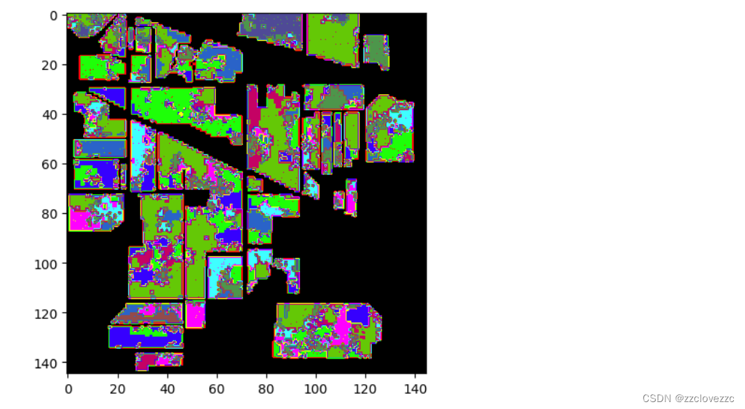
for i in range(height):for j in range(width):if int(y[i,j]) == 0:continueelse :image_patch = X[i:i+patch_size, j:j+patch_size, :]image_patch = image_patch.reshape(1,image_patch.shape[0],image_patch.shape[1], image_patch.shape[2], 1)X_test_image = torch.FloatTensor(image_patch.transpose(0, 4, 3, 1, 2)).to(device)prediction = net(X_test_image)prediction = np.argmax(prediction.detach().cpu().numpy(), axis=1)outputs[i][j] = prediction+1if i % 20 == 0:print('... ... row ', i, ' handling ... ...')

predict_image = spectral.imshow(classes = outputs.astype(int),figsize =(5,5))

分别进行了三组，SoftMax，LogSoftmax，LogSoftmax+BN，测试结果如下

SoftMax

LogSoftmax

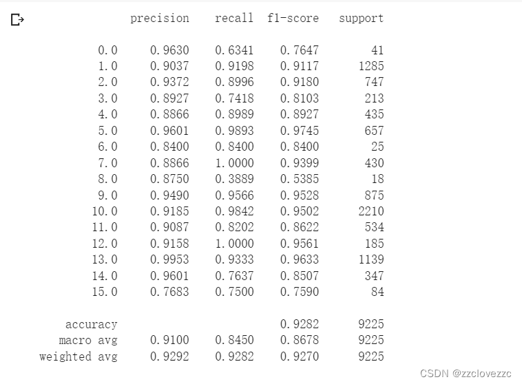
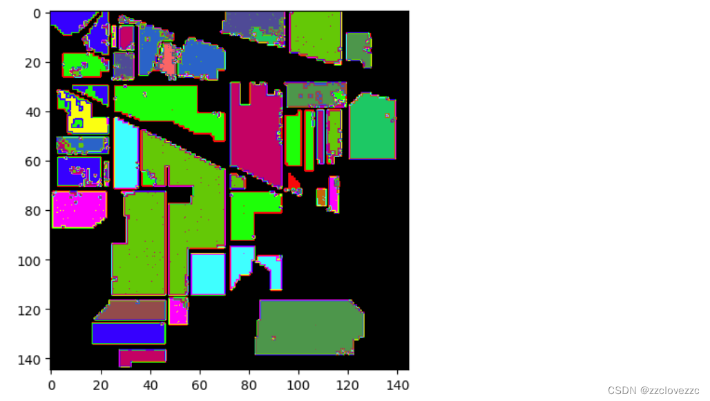
  LogSoftmax+BN

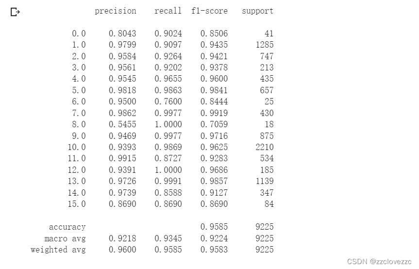
  由实验结果可知使用logsoftmax代替softmax之后，效果显著提升，因为它能够解决函数overflow和underflow，加快运算速度，提高数据稳定性。BN对图像来说类似于一种对比度的拉伸，其色彩的分布都会被归一化，会破坏了图像原本的对比度信息，并且图像分类不需要保留图像的对比度信息，利用图像的结构信息就可以完成分类，所以Batch Norm反而降低了训练难度，甚至一些不明显的结构，在Batch Norm后也会被凸显出来（对比度被拉开了）。

第二部分 问题思考

1.3D卷积和2D卷积的区别
1）2D卷积和3D卷积的主要区别在于卷积核和输入数据的维度不同。2D卷积的卷积核和输入数据都是二维的，而3D卷积的卷积核和输入数据都是三维的。这意味着3D卷积可以同时考虑空间和时间（或深度）上的信息，而2D卷积只能考虑空间上的信息。
2）2D卷积和3D卷积的另一个区别在于计算量和参数量不同。由于3D卷积涉及更多的维度，因此它需要更多的计算资源和存储空间，也更容易导致过拟合。因此，在实际应用中，需要根据不同的任务和数据选择合适的卷积类型。

2.训练HybridSN，然后多测试几次，会发现每次分类的结果都不一样，请思考为什么？

1）HybridSN 模型使用了 Dropout 层，这是一种防止过拟合的技术，它会随机地在训练过程中失活一些神经元，从而减少模型对特定数据的依赖。
2)  HybridSN 模型使用了随机初始化的权重参数，它会根据一定的分布或范围给每个参数赋予一个随机值。
3)  HybridSN 模型使用了 Adam 优化器，这是一种基于梯度下降的优化算法，它会根据梯度的变化动态地调整学习率。每次训练时，模型的更新步长都会不同，导致最优解的寻找过程有所波动。

3.如果想要进一步提升高光谱图像的分类性能，可以如何改进？

1)  用更多的训练数据，或者使用数据增强技术，来增加模型的泛化能力和鲁棒性，从而减少过拟合和噪声的影响。
2)  用更合适的损失函数，例如交叉熵损失或者对比损失，来优化模型的分类性能，从而提高分类准确率和召回率。

4.depth-wise conv和分组卷积有什么区别与联系？

联系：

1）depth-wise conv 和分组卷积都是一种减少参数量和计算量的卷积方式，它们都是将输入的特征图按照通道进行分组，然后对每个组进行独立的卷积操作。
2）depth-wise conv 是一种特殊的分组卷积，它的分组数等于输入特征图的通道数，也就是每个通道单独进行卷积，而不与其他通道共享卷积核。
3）分组卷积和 depth-wise conv 都需要与 point-wise conv （即 1x1 的卷积）结合使用，以实现跨通道的信息融合和输出维度的调整。

区别：

1）分组卷积可以看作是通道稀疏连接的方式，它可以增加特征图之间的多样性和互补性，从而提高模型的表达能力。depth-wise conv 可以看作是空间和通道的完全分离，它可以捕捉每个通道内部的特征，从而提高模型的效率。

4.SENet 的注意力是不是可以加在空间位置上？
  SENet 的注意力机制可以加在空间位置上，即对每个像素点或区域进行权重分配，从而增强感兴趣的区域，抑制背景噪声 。

5.在 ShuffleNet 中，通道的 shuffle 如何用代码实现？

  只需要对特征图进行维度重排即可。假设将输入层分为 g 组，总通道数为 g × n，首先将通道那个维度拆分为 (g, n) 两个维度，然后将这两个维度转置变成 (n, g) ，最后重新 reshape 成一个维度 g×n 

def channel_shuffle(x: Tensor, groups: int) -> Tensor:batch_size, num_channels, height, width = x.size()channels_per_group = num_channels // groups# reshape# [batch_size, num_channels, height, width] -> [batch_size, groups, channels_per_group, height, width]x = x.view(batch_size, groups, channels_per_group, height, width)x = torch.transpose(x, 1, 2).contiguous()# flattenx = x.view(batch_size, -1, height, width)return x

本文来自互联网用户投稿，文章观点仅代表作者本人，不代表本站立场，不承担相关法律责任。如若转载，请注明出处。 如若内容造成侵权/违法违规/事实不符，请点击【内容举报】进行投诉反馈！