学术讲座: 多标签主动学习之 MASP
摘要: 本贴解读我们的刚录用的论文 Xue-Yang Min, Kun Qian, Ben-Wen Zhang, Guojie Song, and Fan Min, Multi-label active learning through serial-parallel neural networks, Knowledge-Based Systems (2022) pp. xxx. doi: yyy.
1. 问题描述
从简单到复杂, 为多标签学习、多标签主动学习.
1.1 多标签学习
这里是多标签学习专题讲座.
定义1. 多标签数据为一个二元组:
S = ( X , Y ) , (1) S = (\mathbf{X}, \mathbf{Y}), \tag{1} S=(X,Y),(1)
其中
- X = ( x 1 , x 2 , … , x N ) T = ( x i j ) N × M \mathbf{X} = (\mathbf{x}_1, \mathbf{x}_2, \dots, \mathbf{x}_N)^{\mathrm{T}} = (x_{ij})_{N \times M} X=(x1,x2,…,xN)T=(xij)N×M 为条件属性矩阵;
- Y = ( y 1 , y 2 , … , y N ) T = ( y i j ) N × L \mathbf{Y} = (\mathbf{y}_1, \mathbf{y}_2, \dots, \mathbf{y}_N)^{\mathrm{T}} = (y_{ij})_{N \times L} Y=(y1,y2,…,yN)T=(yij)N×L 为标签矩阵;
- N N N 为对象数;
- M M M 为条件属性数;
- L L L 为标签数;
- y i j = 1 y_{ij} = 1 yij=1 表示 x i \mathbf{x}_i xi 具有标签 j j j, y i j = − 1 y_{ij} = -1 yij=−1 表示不具有.
多标签学习就是根据 S S S 建立一个分类器, 并用于未知实例的预测.
1.2 带缺失标签的多标签学习
y i j = 0 y_{ij} = 0 yij=0 表示 x i \mathbf{x}_i xi 是否具有标签 j j j.
实际数据多半具有标签缺失的特点, 在很多情况下缺失还非常严重.
1.3 多标签主动学习
允许学习器进行标签的查询. 作为一种最简单的场景, , 需要进行一定轮次的查询才能构建良好的学习器.
问题 1. 有限预算的冷启动多标签学习。
输入: X \mathbf{X} X, Y \mathbf{Y} Y (仅专家知道), 查询上限 Q Q Q;
输出: 预测模型 Θ : R M → { − 1 , + 1 } L \Theta: \mathbb{R}^M \to \{-1, +1\}^L Θ:RM→{−1,+1}L, 查询的 实例-标签对集合 Q \mathbf{Q} Q.
优化目标: Θ \Theta Θ 的预测精度.
说明:
- 初始状态下所有标签都缺失. 这样利于不同算法的比较.
- 基于池的查询, 即 实例-标签对 的查询没有顺序限制. 这与 在线主动学习 不同.
- 批量查询. 可以节约时间.
- 查询量 Q Q Q 预先指定. 这是专家工作量.
- 在未见实例上测试. 不同于直推机.
2. 学习模型
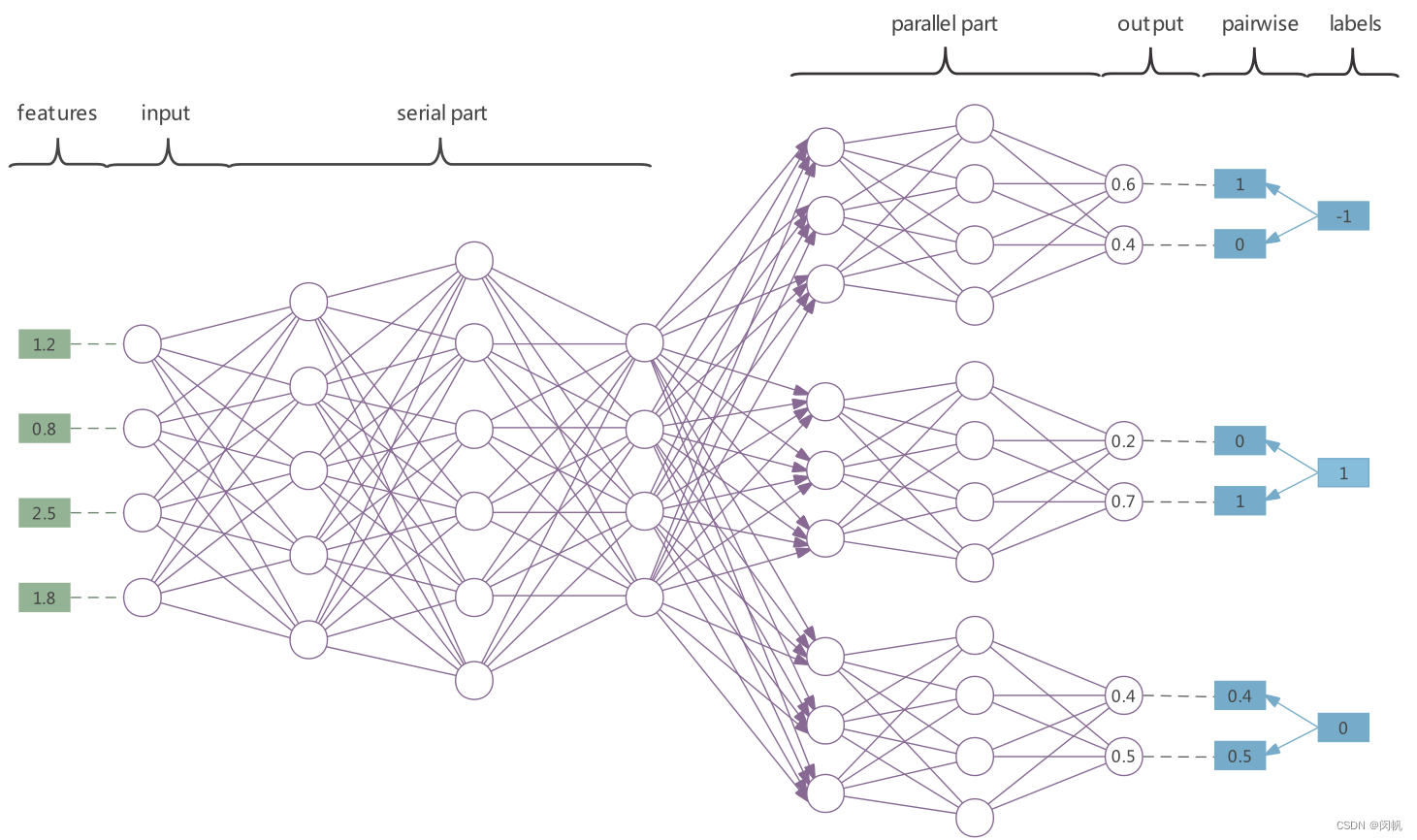
- 串行部分用于属性提取.
- 也用于应对标签相关性. - 并行部分用于预测.
- 成对的预测提供更稳定的结果.
- 对于缺失标签, 就不进行相应的惩罚.
- 预测的时候既可以直接获得标签, 又可以通过 softmax 转换为一个概率值. - 简单起见, 未画出偏移量.
- 为适应 GPU, 每层节点数为 64, 128 等. GPU 真香呀!
- 定制一个网络很方便. Python 也香呀!
如果需要实型的预测, 就使用 softmax 函数:
y ^ i k ′ = exp g k + ( f ( x i ) ) exp g k + ( f ( x i ) ) + exp g k − ( f ( x i ) ) . \hat{y}'_{ik} = \frac{\exp g_k^+(f(\mathbf{x}_i))}{\exp g_k^+(f(\mathbf{x}_i)) + \exp g_k^-(f(\mathbf{x}_i))}. y^ik′=expgk+(f(xi))+expgk−(f(xi))expgk+(f(xi)).
class ParallelAnn(nn.Module):"""Parallel ANN.This class handles the parallel part."""def __init__(self, para_parallel_layer_num_nodes: list = None, para_activators: str = "s" * 100):super().__init__()temp_model = []for i in range(len(para_parallel_layer_num_nodes) - 1):temp_input = para_parallel_layer_num_nodes[i]temp_output = para_parallel_layer_num_nodes[i + 1]temp_linear = nn.Linear(temp_input, temp_output)temp_model.append(temp_linear)temp_model.append(get_activator(para_activators[i]))self.model = nn.Sequential(*temp_model)def forward(self, para_input: torch.tensor = None):temp_output = self.model(para_input)return temp_outputclass MultiLabelAnn(nn.Module):"""Multi-label ANN.This class handles the whole network."""def __init__(self, para_dataset: MultiLabelData = None, para_full_connect_layer_num_nodes: list = None,para_parallel_layer_num_nodes: list = None, para_learning_rate: float = 0.01,para_mobp: float = 0.6, para_activators: str = "s" * 100, para_device=None):super().__init__()self.dataset = para_datasetself.num_parts = self.dataset.num_labelsself.num_layers = len(para_full_connect_layer_num_nodes) + len(para_parallel_layer_num_nodes)self.learning_rate = para_learning_rateself.mobp = para_mobpself.device = para_deviceself.skip_count = 0 # For cost-sensitive learning.temp_model = []for i in range(len(para_full_connect_layer_num_nodes) - 1):temp_input = para_full_connect_layer_num_nodes[i]temp_output = para_full_connect_layer_num_nodes[i + 1]temp_linear = nn.Linear(temp_input, temp_output)temp_model.append(temp_linear)temp_model.append(get_activator(para_activators[i]))self.full_connect_model = nn.Sequential(*temp_model)temp_parallel_activators = para_activators[len(para_full_connect_layer_num_nodes) - 1:]self.parallel_model = [ParallelAnn(para_parallel_layer_num_nodes, temp_parallel_activators).to(self.device)for _ in range(self.dataset.num_labels)]self.my_optimizer = torch.optim.Adam(itertools.chain(self.full_connect_model.parameters(),*[model.parameters() for model in self.parallel_model]),lr=para_learning_rate)self.my_loss_function = nn.MSELoss().to(para_device)def forward(self, para_input: np.ndarray = None):temp_input = torch.tensor(para_input, dtype=torch.float).to(self.device)temp_inner_output = self.full_connect_model(temp_input)temp_inner_output = [model(temp_inner_output) for model in self.parallel_model]temp_output = temp_inner_output[0]for i in range(len(temp_inner_output) - 1):temp_output = torch.cat((temp_output, temp_inner_output[i + 1]), -1)return temp_output
3. 学习场景
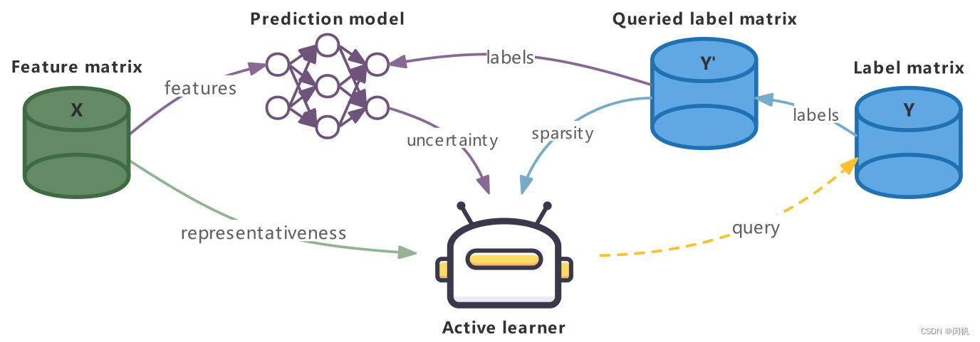
- X \mathbf{X} X 已知.
- Y ′ \mathbf{Y}' Y′ 通过查询 Y \mathbf{Y} Y 获得. 简化起见未画出人类专家.
- 使用 X \mathbf{X} X 和 Y ′ \mathbf{Y}' Y′ 训练网络.
4. 实例-标签对选择方案
主动学习的核心就是进行实例-标签对选择.
4.1 实例代表性 (根据 X \mathbf{X} X 计算).
参见 日撸 Java 三百行第 66 天
实例密度:
ρ i = ∑ j ≠ i e − ( d i j d c ) 2 , \rho_i = \sum_{j \neq i} e^{- \left(\frac{d_{ij}}{d_c}\right)^2}, ρi=j=i∑e−(dcdij)2,
其中 d i j d_{ij} dij 是 x i \mathbf{x}_i xi 与 x j \mathbf{x}_j xj 之间的距离, d c d_c dc 为一个用户设置的阈值. 如果数据已经归一化, 可设置 d c = 0.1 d_c = 0.1 dc=0.1.
实例到父节点的距离:
δ i = min ρ j > ρ i d i j . \delta_i = \min_{\rho_j > \rho_i} d_{ij}. δi=ρj>ρimindij.
实例代表性:
γ i = ρ i δ i . \gamma_i = \rho_i \delta_i. γi=ρiδi.
4.2 标签稀疏性 (根据 Y ′ \mathbf{Y}' Y′ 计算).
ψ k = 1 − ∣ Q ∩ { 1 , 2 , … , N } × { k } ∣ N . \psi_k = 1 - \frac{\vert \mathbf{Q} \cap \{1, 2, \dots, N\} \times \{k\} \vert}{N}. ψk=1−N∣Q∩{1,2,…,N}×{k}∣.
4.3 标签不确定性 (根据成对的预测值计算).
η ( i , k ) = { 0 , if y i k is queried; 1 − ∣ g k − ( f ( x i ) ) − g k + ( f ( x i ) ) ∣ , otherwise. \eta(i, k) = \left\{\begin{array}{ll} 0, & \textrm{ if } y_{ik} \textrm{ is queried;}\\ 1 - \left\vert g_k^-(f(\mathbf{x}_i)) - g_k^+(f(\mathbf{x}_i)) \right\vert, & \textrm{ otherwise.}\end{array}\right. η(i,k)={0,1−∣∣gk−(f(xi))−gk+(f(xi))∣∣, if yik is queried; otherwise.
5. 小结
未完待续.
本文来自互联网用户投稿,文章观点仅代表作者本人,不代表本站立场,不承担相关法律责任。如若转载,请注明出处。 如若内容造成侵权/违法违规/事实不符,请点击【内容举报】进行投诉反馈!